Difference between revisions of "Plot gallery"
| (29 intermediate revisions by 7 users not shown) | |||
| Line 2: | Line 2: | ||
Please add your with <code>slxfig</code> created plots! Preferably format: clickable image of your final product, leading to the s-lang code (with or without comments). When uploading pictures, please don't forget to give them a '''unique''' name, as they are all stored in one directory. | Please add your with <code>slxfig</code> created plots! Preferably format: clickable image of your final product, leading to the s-lang code (with or without comments). When uploading pictures, please don't forget to give them a '''unique''' name, as they are all stored in one directory. | ||
| + | |||
| + | A cool website for generating color-blind friendly patterns: https://coolors.co/121619-2d4739-09814a-bcb382-e5c687. You can set the colors just by using the hex codes in xfig or tikz. | ||
=== Mike's Fancy Plots === | === Mike's Fancy Plots === | ||
| Line 43: | Line 45: | ||
=== Colorful Cyg X-1 lightcurves === | === Colorful Cyg X-1 lightcurves === | ||
| − | [[File:lc_cygx1.png|500px|link= | + | [[File:lc_cygx1.png|500px|link=Lightcurve_Cygx1_(xfig_example)]] |
Combining ''RXTE''-ASM, ''Swift''-BAT and ''MAXI'' lightcurves of Cyg X-1 in one plot. The ''RXTE'' lightcurve is color-coded for the low/hard (blue) and the high/soft (red) state. The colors for ''Swift'' are the same as for ''RXTE'' at the same time, or, when the ''RXTE'' lightcurve stops, as during times with similar count rates. ''MAXI'' has its own scale from black (low/hard) to grey (high/soft). Additionally, times of Chandra observations won by our group are indicated (AO13 was scheduled but then canceled). — ''[mailto:Natalie.Hell@sternwarte.uni-erlangen.de Natalie Hell] & [mailto:Ivica.Miskovicova@sternwarte.uni-erlangen.de Ivica Miškovičová]'' | Combining ''RXTE''-ASM, ''Swift''-BAT and ''MAXI'' lightcurves of Cyg X-1 in one plot. The ''RXTE'' lightcurve is color-coded for the low/hard (blue) and the high/soft (red) state. The colors for ''Swift'' are the same as for ''RXTE'' at the same time, or, when the ''RXTE'' lightcurve stops, as during times with similar count rates. ''MAXI'' has its own scale from black (low/hard) to grey (high/soft). Additionally, times of Chandra observations won by our group are indicated (AO13 was scheduled but then canceled). — ''[mailto:Natalie.Hell@sternwarte.uni-erlangen.de Natalie Hell] & [mailto:Ivica.Miskovicova@sternwarte.uni-erlangen.de Ivica Miškovičová]'' | ||
| Line 60: | Line 62: | ||
=== Linear-Logarithmic Axis === | === Linear-Logarithmic Axis === | ||
| − | [[File:lin_log_axis.png|300px|link= | + | [[File:lin_log_axis.png|300px|link=Lin log axis (xfig example)]] Another example of a user defined axis (partially linear and logarithmic). — ''[mailto:Moritz.Boeck@sternwarte.uni-erlangen.de Moritz Boeck]'' |
=== Plotting images with world coordinates === | === Plotting images with world coordinates === | ||
| Line 75: | Line 77: | ||
=== Monster Lightcurve Plot === | === Monster Lightcurve Plot === | ||
| − | [[File:monster_lightcurve_vg.png|400px|link= | + | [[File:monster_lightcurve_vg.png|400px|link=Monsterlightcurve (xfig example)]] |
Lightcurves from all all-sky monitors & time of individual pointed RXTE observations of Cyg X-1. — ''[mailto:Victoria.Grinberg@sternwarte.uni-erlangen.de Victoria Grinberg]'' | Lightcurves from all all-sky monitors & time of individual pointed RXTE observations of Cyg X-1. — ''[mailto:Victoria.Grinberg@sternwarte.uni-erlangen.de Victoria Grinberg]'' | ||
| Line 101: | Line 103: | ||
=== Insets as zoom-ins === | === Insets as zoom-ins === | ||
| − | [[File:gx304batlcobs.png|300px|link= | + | [[File:gx304batlcobs.png|300px|link=GX304batlcobs_(xfig_example)]] |
Plotting the BAT-lightcurve of a source and adding zooms into the lightcurve showing the available observations. —'' | Plotting the BAT-lightcurve of a source and adding zooms into the lightcurve showing the available observations. —'' | ||
[mailto:Matthias.Kuehnel@sternwarte.uni-erlangen.de Matthias Kühnel]'' | [mailto:Matthias.Kuehnel@sternwarte.uni-erlangen.de Matthias Kühnel]'' | ||
| Line 116: | Line 118: | ||
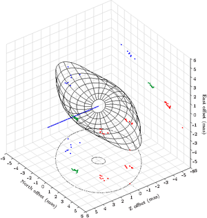
=== 3D Maser Disk === | === 3D Maser Disk === | ||
| − | [[File:disk_map.png|300px|link= | + | [[File:disk_map.png|300px|link=3D_Maser_Disk_(xfig_example)]] |
3D Maser disk and projections on 2D. —'' | 3D Maser disk and projections on 2D. —'' | ||
[mailto:Eugenia.Litzinger@sternwarte.uni-erlangen.de Eugenia Litzinger]'' | [mailto:Eugenia.Litzinger@sternwarte.uni-erlangen.de Eugenia Litzinger]'' | ||
| Line 126: | Line 128: | ||
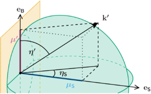
=== Plotting in 3D, simple === | === Plotting in 3D, simple === | ||
| − | [[File:object3dsimple.png|300px|link= | + | [[File:object3dsimple.png|300px|link=Object3dsimple (xfig example)]] |
An simple example how to create a 3D plot using vector transformations.'' | An simple example how to create a 3D plot using vector transformations.'' | ||
[mailto:sebastian.falkner@fau.de Sebastian Falkner]'' | [mailto:sebastian.falkner@fau.de Sebastian Falkner]'' | ||
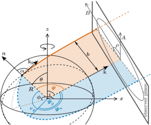
=== Plotting in 3D === | === Plotting in 3D === | ||
| − | [[File:object3d.png|300px|link= | + | [[File:object3d.png|300px|link=Object3d (xfig example)]] |
An example how to create a 3D plot using vector transformations.'' | An example how to create a 3D plot using vector transformations.'' | ||
[mailto:sebastian.falkner@fau.de Sebastian Falkner]'' | [mailto:sebastian.falkner@fau.de Sebastian Falkner]'' | ||
| Line 137: | Line 139: | ||
=== Calculating and plotting orbits in 3D === | === Calculating and plotting orbits in 3D === | ||
| − | [[File:orbit3d.png|300px|link= | + | [[File:orbit3d.png|300px|link=3D orbit plots (xfig example)]] |
Calculation and plots of orbits in 3D'' | Calculation and plots of orbits in 3D'' | ||
[mailto:matthias.kuehnel@sternwarte.uni-erlangen.de Matthias Kuehnel]'' | [mailto:matthias.kuehnel@sternwarte.uni-erlangen.de Matthias Kuehnel]'' | ||
| Line 155: | Line 157: | ||
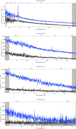
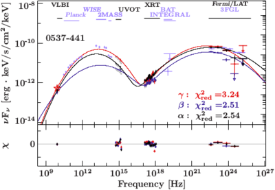
=== Multipanel spectral model decomposition === | === Multipanel spectral model decomposition === | ||
| − | [[File:multipanel_decomposition.png|400px|link= | + | [[File:multipanel_decomposition.png|400px|link=Model decomp (xfig example)]] |
Spectral model decompositions of a whole sample using multiplot. Compact and flexible code thanks to some clean file structuring and efficiently placed loops.—''[mailto:marco.fink@fau.de Marco Fink]'' | Spectral model decompositions of a whole sample using multiplot. Compact and flexible code thanks to some clean file structuring and efficiently placed loops.—''[mailto:marco.fink@fau.de Marco Fink]'' | ||
| Line 192: | Line 194: | ||
[[Category:SLxfig]] | [[Category:SLxfig]] | ||
[[Category:Isis / Slang]] | [[Category:Isis / Slang]] | ||
| + | |||
| + | === Skymap with error circles === | ||
| + | [[File:Skymapcirclegr.png|700px|link=Plot_skymap_(xfig_example)]] | ||
| + | |||
| + | How to plot a circles in spherical coordinates in a Hammer-Aitoff projection. (Or: how to plot the intersection of a sphere with a plane) | ||
| + | [mailto:Felicia.Krauss@fau.de Felicia Krauss]'' | ||
| + | |||
| + | === Plot data over different range sections === | ||
| + | [[File:plot_with_gaps_jjs.png|300px|link=Plot_data_with_gaps_(xfig_example)]] | ||
| + | |||
| + | A simple example on how to plot data over a range with gaps, inserting visible markers to indicate these gaps. ''— [mailto:jakob.stierhof@fau.de Jakob Stierhof]'' | ||
| + | |||
| + | === Plot geospatial data with shapelib === | ||
| + | [[File:plot_world_jjs.png|800px|link=Plot_geospatial_data_(xfig_example)]] | ||
| + | |||
| + | [[File:plot_world_vector_jjs.png|800px|link=Plot_geospatial_data_(xfig_example)]] | ||
| + | |||
| + | An exemplary use of the slang interface to the lightweight shapelib library. The library allows to read in ESRI shape files a common format for geospatial data representation. The slang wrapper is in a very early phase and together with the not very error prone shapelib c library there is lots of errors ahead of you (okay, mostly it's my fault). For example, if you try to load a file that does not exist the wrapper does not crash nicely bad faces you with a segfault. You have been warned! ''— [mailto:jakob.stierhof@fau.de Jakob Stierhof]'' | ||
| + | |||
| + | === Coloredcoded scatter plot === | ||
| + | [[File:my_very_cool_colorcode.png|500px|link=Colorcoded_scatter_plot]] | ||
| + | Colorcoded scatter plot ''— [mailto:philipp.ph.weber@fau.de Philipp Weber] or [mailto:steven.haemmerich@fau.de Steven Hämmerich]'' | ||
| + | |||
| + | === Plot marginal and joint probabilities === | ||
| + | |||
| + | [[File:Distribution_matrix.png|500px|link=Plot_marginal_and_joing_probabilities]] | ||
| + | |||
| + | Visualize the distribution of something in a nice triangle using one function (from the isisscripts)! ''- [mailto:jakob.stierhof@fau.de Jakob Stierhof] | ||
| + | |||
| + | = Remeis tikz plot gallery = | ||
| + | |||
| + | === Plot continuum models with varying parameters === | ||
| + | |||
| + | [[File:continuum_functions.png|500px|link=Continuum functions (tikz plot)]] | ||
| + | |||
| + | Visualisation of common continuum models used for the spectra of accreting neutron stars. [[:File:Continuum_functions.pdf|Version in better resolution]] Author: [mailto:nicolas.zalot@fau.de Nicolas Zalot] | ||
| + | |||
| + | === Display of available color palettes and maps === | ||
| + | |||
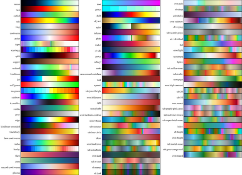
| + | [[File:Color-palettes-isisscripts.png|500px|link=For all your color needs!]] | ||
| + | [[File:Color-maps-isisscripts.png|500px|link=For all your color needs!]] | ||
| + | |||
| + | Simple iterator script to display color maps and color palettes using the isisscripts color interface. ''- [mailto:jakob.stierhof@fau.de Jakob Stierhof] | ||
Latest revision as of 10:08, 13 February 2024
Remeis X-fig plot gallery
Please add your with slxfig created plots! Preferably format: clickable image of your final product, leading to the s-lang code (with or without comments). When uploading pictures, please don't forget to give them a unique name, as they are all stored in one directory.
A cool website for generating color-blind friendly patterns: https://coolors.co/121619-2d4739-09814a-bcb382-e5c687. You can set the colors just by using the hex codes in xfig or tikz.
Mike's Fancy Plots
 Plotting spectra in the way of Mike's fancy plots
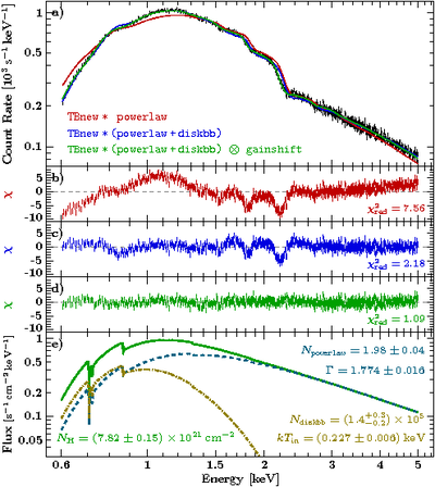
Plotting Model Components
 Plotting individual model components
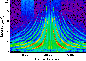
Color-coded maps with png and xfig
How to plot a color-coded map (landscape) using png and xfig
Two-dimensional histograms
 banana-plot with coordinate system —Manfred Hanke
Compounds and multiplots
 Compounds and multi-panel plots —Manfred Hanke
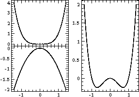
parameter-space sketches
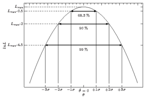
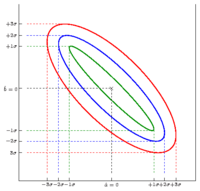 Simple plots to sketch the meaning of sigma-values in 1-dim or 2-dim chi-squared parameter spaces. (MB: Be aware that the n-sigma projection of 2D contours on one parameter differs from the n-sigma levels obtained for only this parameter (1D), as the delta-chi^2 (or delta statistic) depends on the number of parameters.)
Author — Tobias Beuchert 2013-01-07 13:41
Simple plots to sketch the meaning of sigma-values in 1-dim or 2-dim chi-squared parameter spaces. (MB: Be aware that the n-sigma projection of 2D contours on one parameter differs from the n-sigma levels obtained for only this parameter (1D), as the delta-chi^2 (or delta statistic) depends on the number of parameters.)
Author — Tobias Beuchert 2013-01-07 13:41
Orbit plot
 Orbit plot of GX 301-2, including the average ASM lightcurve folded on the orbit. Version in better resolution (pdf). Author — Felix Fürst 2012-05-23 17:47
4 colorful landscapes
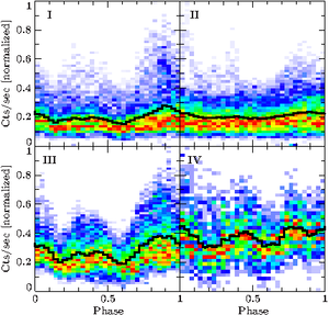 Color-coded maps of count-rate distribution in the pulse-profile for different epochs. Very similar to what is shown in an example: plotting color-coded maps with the png and xfig modules. Writing out the PNG with a separate routine is not neccessary anymore I think, code is a little oldish. Author — Felix Fürst 2012-05-23 17:55
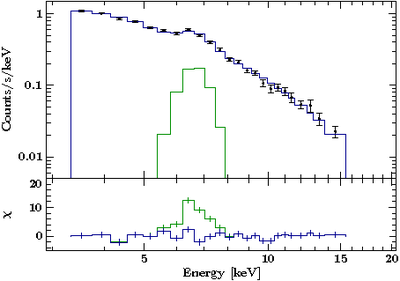
Contour plot
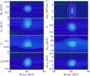 Contour plot of the Cyclo line energy of XTE J1946+274. — Sebastian Mueller 2012-05-30 15:53
2D image contours
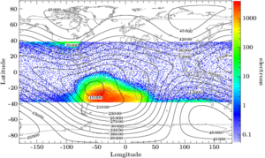 Map (2D histogram) of the South Atlantic Anomaly (SAA) overplotted with iso-magnetic field lines of the Earth's magnetic field. — Natalie Hell
Colorful Cyg X-1 lightcurves
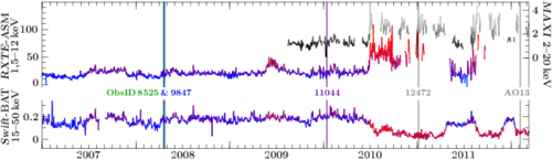
Combining RXTE-ASM, Swift-BAT and MAXI lightcurves of Cyg X-1 in one plot. The RXTE lightcurve is color-coded for the low/hard (blue) and the high/soft (red) state. The colors for Swift are the same as for RXTE at the same time, or, when the RXTE lightcurve stops, as during times with similar count rates. MAXI has its own scale from black (low/hard) to grey (high/soft). Additionally, times of Chandra observations won by our group are indicated (AO13 was scheduled but then canceled). — Natalie Hell & Ivica Miškovičová
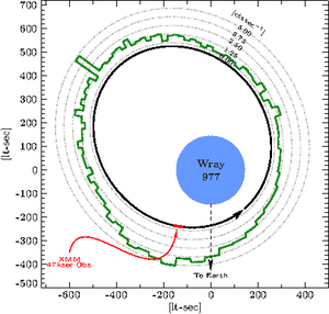
Chandra coverage of Cyg X-1
Plot of the orbital coverage of Cyg X-1 with Chandra observations, including an example of how to calculate Roche lobes with isis. —Manfred Hanke
Wind structure in Cyg X-1
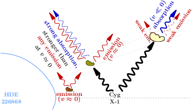
You may not know, but you can draw basically anything with slxfig! Here is a very nice example from Manfred's PhD thesis (see Fig. 2.62 in there for an interpretation), describing our idea of the wind structure in the Cyg X-1 system.
The plot includes a couple of very nice tricks. Slxfig provides a function to draw photons. The example also shows how to add existing eps files to the figure, and how to add your own functions to the structure saving the xfig plot. — Manfred Hanke
Linear-Logarithmic Axis
 Another example of a user defined axis (partially linear and logarithmic). — Moritz Boeck
Plotting images with world coordinates
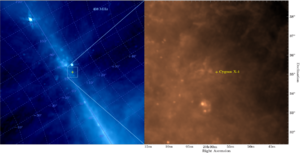 408 MHz and IRAS images of regions centered at the position of Cygnus X-1. The WCS module is used to show sky coordinates (galactic coordinate grid on the left, RA-DEC axis labels on the right)— Moritz Boeck
Skyplot of source positions
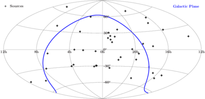 Random source positions shown in an Aitoff projection of the sky in RA and DEC. The Galactic Plane is highlighted. — Moritz Boeck
Electromagnetic Spectrum
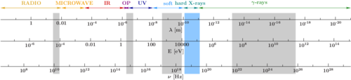 Electromagnetic spectrum in energy, frequency and wavelength. Satellite energy ranges marked.
Original Script by Cornelia Müller
— Felicia Krauß
Electromagnetic spectrum in energy, frequency and wavelength. Satellite energy ranges marked.
Original Script by Cornelia Müller
— Felicia Krauß
Monster Lightcurve Plot
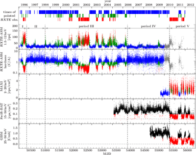 Lightcurves from all all-sky monitors & time of individual pointed RXTE observations of Cyg X-1. — Victoria Grinberg
Periodic Table
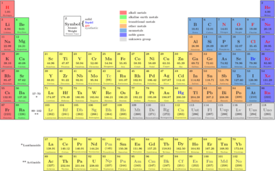 Draw your own periodic table in only ~120 lines of code. Data is taken from the X-ray Data Booklet 2009. —
Natalie Hell
Draw your own periodic table in only ~120 lines of code. Data is taken from the X-ray Data Booklet 2009. —
Natalie Hell
Relativistic photon trajectory
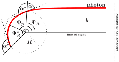 Sketch of a relativistic photon trajectory. NOTE: "lbscripts" are required to execute the script. The path is set in the Script correctly, otherwise please contact me. — Sebastian Falkner
Atomic processes
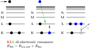 Make sketches of atomic processes such as di-electronic recombination (DR). Other possibilities include radiative recombination, auto-ionization, photo-ionization, ... —
Natalie Hell
Make sketches of atomic processes such as di-electronic recombination (DR). Other possibilities include radiative recombination, auto-ionization, photo-ionization, ... —
Natalie Hell
Simple inset
Insets and shaded regions
 Plotting the BAT-lightcurve of a source and shading specific regions as well as labeling them. Furthermore, adding an inset plot showing an epoch folding result here. —
Matthias Kühnel
Plotting the BAT-lightcurve of a source and shading specific regions as well as labeling them. Furthermore, adding an inset plot showing an epoch folding result here. —
Matthias Kühnel
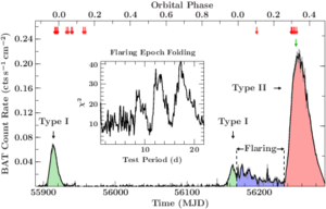
Insets as zoom-ins
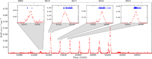 Plotting the BAT-lightcurve of a source and adding zooms into the lightcurve showing the available observations. —
Matthias Kühnel
Plotting the BAT-lightcurve of a source and adding zooms into the lightcurve showing the available observations. —
Matthias Kühnel
Hertzsprung-Russell diagram
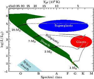 A schematic Hertzsprung-Russell diagram —
Andreas Irrgang
A schematic Hertzsprung-Russell diagram —
Andreas Irrgang
Colored data points
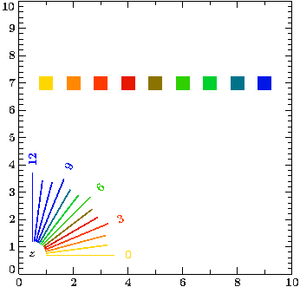 "Speedometer"-like colormap for data points —
Andreas Irrgang
"Speedometer"-like colormap for data points —
Andreas Irrgang
3D Maser Disk
 3D Maser disk and projections on 2D. —
Eugenia Litzinger
3D Maser disk and projections on 2D. —
Eugenia Litzinger
Angstrom and keV axes done properly in the same plot (axis coordinate transformation)
 Simple but extremely useful axis transformation; works both ways in spite of the name —
Grinberg
Simple but extremely useful axis transformation; works both ways in spite of the name —
Grinberg
Plotting in 3D, simple
 An simple example how to create a 3D plot using vector transformations.
Sebastian Falkner
An simple example how to create a 3D plot using vector transformations.
Sebastian Falkner
Plotting in 3D
 An example how to create a 3D plot using vector transformations.
Sebastian Falkner
An example how to create a 3D plot using vector transformations.
Sebastian Falkner
Calculating and plotting orbits in 3D
 Calculation and plots of orbits in 3D
Matthias Kuehnel
Calculation and plots of orbits in 3D
Matthias Kuehnel
It also defines additional TeX commands and packages for plotting purposes, such as using no bold face.
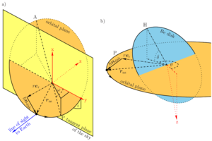
VLBI coordinates in 3D
 Displaying VLBI coordinates in 3D
Tobias Beuchert
Displaying VLBI coordinates in 3D
Tobias Beuchert
Plotting a fit model
How to plot a fit model in xfig to extend beyond the data. Felicia Krauss
Multipanel spectral model decomposition

Spectral model decompositions of a whole sample using multiplot. Compact and flexible code thanks to some clean file structuring and efficiently placed loops.—Marco Fink
Chi²-distribution and CDF
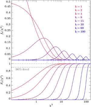
The Chi²-distribution and its according cumulative distribution function for a large number of degrees of freedom. Confidence levels are indicated in the CDF. Feel free to use it in your thesis.—Marco Fink
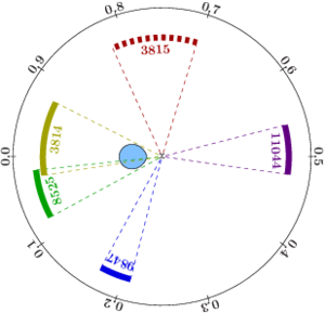
Polar Plot
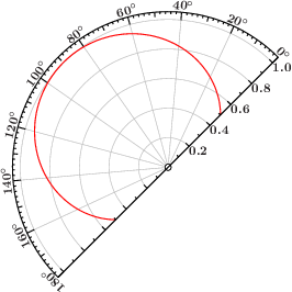
In the isisscripts there is a function 'xfig_polarplot_new, with which provides an easy way to plot an individual adjustable polar plot. This plot is just one very simple example, for more information see 'isis> help xfig_polarplot_new'.—Sebastian Falkner
Xfig plot image
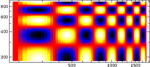
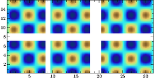
Other than the %plot_png function of the xfig_plot structure this function aims to plot images with a (given) ARBITRARY x/y-grid in a correct way (NOTE that .plot_png does not care for x/y values!). This also allows to plot images with logarithmic scales without any problems! In addition it is easy to plot gabbed images by just giving the x and y grid as bin_lo and bin_hi.
These plots are just two very simple examples, for more information see 'isis> help xfig_plot_image'.—Sebastian Falkner
Xfig plot colormap
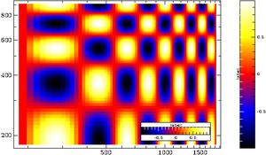
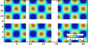
The function 'xfig_plot_colormap' creates a horizontal, vertical colormap/colorscale for a given image. For more information see 'isis> help xfig_plot_colormap'.—Sebastian Falkner
Skymap with error circles
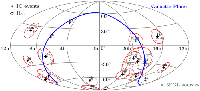
How to plot a circles in spherical coordinates in a Hammer-Aitoff projection. (Or: how to plot the intersection of a sphere with a plane) Felicia Krauss
Plot data over different range sections
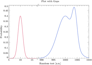
A simple example on how to plot data over a range with gaps, inserting visible markers to indicate these gaps. — Jakob Stierhof
Plot geospatial data with shapelib
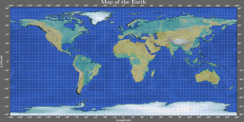
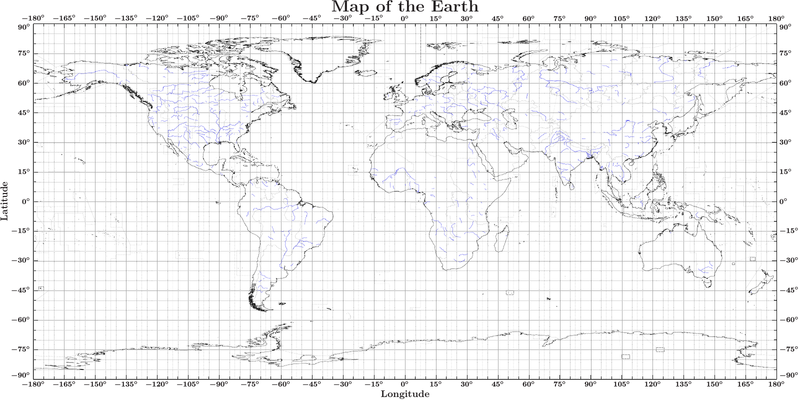
An exemplary use of the slang interface to the lightweight shapelib library. The library allows to read in ESRI shape files a common format for geospatial data representation. The slang wrapper is in a very early phase and together with the not very error prone shapelib c library there is lots of errors ahead of you (okay, mostly it's my fault). For example, if you try to load a file that does not exist the wrapper does not crash nicely bad faces you with a segfault. You have been warned! — Jakob Stierhof
Coloredcoded scatter plot
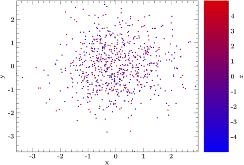 Colorcoded scatter plot — Philipp Weber or Steven Hämmerich
Plot marginal and joint probabilities
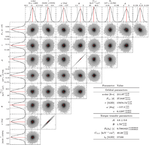
Visualize the distribution of something in a nice triangle using one function (from the isisscripts)! - Jakob Stierhof
Remeis tikz plot gallery
Plot continuum models with varying parameters
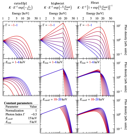
Visualisation of common continuum models used for the spectra of accreting neutron stars. Version in better resolution Author: Nicolas Zalot
Display of available color palettes and maps
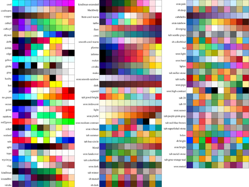
Simple iterator script to display color maps and color palettes using the isisscripts color interface. - Jakob Stierhof