Two-dimensional histograms (xfig example)
example added by Manfred
Similarly to the first example for creating color-coded maps with the SLxfig module, the goal of this one is to produce a color-coded map, but this time, the color-scale represents a density of (a possibly large number of) data points.
ISIS' histogram2d function
Usage
The histogram2d function is used in the following way (see also help("histogram2d")):
num = histogram2d(A, B, Agrid, Bgrid);
A and B have to be Double_Type arrays of the same length,
Agrid and Bgrid have to be Double_Type arrays with monotonically increasing elements.
Now, num[a,b] contains the number of points (A, B)
falling into each 2d-bin defined by the lower bin boundaries Agrid[a] and Bgrid[b], i.e.:
num[a,b] == howmany( (Agrid[a] <= A < Agrid[a+1]) and (Bgrid[b] <= B < Bgrid[b+1]) );
Overflow bins
The last bin in each row or column is an overflow bin whose upper limit is at infinity, i.e.,
 num[-1,b]  ==  howmany( (Agrid[-1] <= A) and (Bgrid[b] <= B < Bgrid[b+1]) );
 num[a,-1]  ==  howmany( (Agrid[a] <= A < Agrid[a+1]) and (Bgrid[-1] <= B) );
and
num[-1,-1] == howmany( (Agrid[-1] <= A) and (Bgrid[-1] <= B) );
If one wants to remove these overflow bins,
one can simply apply the index-array [:-2] (which means "take all elements up to the second last one")
in both dimensions in order to create a smaller two-dimensional array:
num_ = num[ [:-2], [:-2] ];
The last bins corresponding to the reduced 2d-array num_ end now at the same position where the grids end, too:
num_[-1,-1] == num[-2,-2] == howmany( (Agrid[-2] <= A < Agrid[-1]) and (Bgrid[-2] <= B < Bgrid[-1]) );
Before, the grids specified always lower bin boundaries,
but now, the grids have one element more than the correpsonding array-dimensions of num_.
Note that ISIS (one-dimensional) histogram function does not produce an overflow bin.
Order of the indices
The first index of num (called a above) will always correspond
to the first [and third] argument of the histogram2d function (here called A [and Agrid]),
and the second index (b) to the second [and fourth] argument (B [and Bgrid]).
As most functions that operate on two dimensional arrays (like plot_image, png_write, ds9_view, ...)
expect that the first index of the 2d-array to correspond to the y-axis,
whereas only the second index to the x-axis,
one will have to pass the y-data [and -grid] before the x-data [and -grid]:
num = histogram2d(Y, X, Xgrid, Ygrid);
Using two-dimensional histograms
Just as in the previous example, these two dimensional histograms can be transformed into a color-coded image, which can then be included in an xfig plot which adds back the original coordinate system.
A "banana-plot"
In an X-ray gratings spectrometer (Chandra-HETGS, XMM-RGS), the dispersion is not only proportional to the photon's wavelength, but also to the dispersion order. Different orders, however, can be separated with the internal energy resolution of the CCD detector.
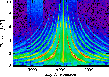
The following example plots the density of events in a position – energy diagram:
Writing the png image
variable evts = fits_read_table("evt2.fits");          % reading a Chandra level-2 event file

variable x_grid = [2300:5700:#320];                    % x position on the detector (320 values)
variable energy_grid = [0:10000:#240];                 % energies in eV (240 values from 0 to 10 keV)

variable num = histogram2d(evts.energy, evts.x,        % the data (Y, X)
                           energy_grid, x_grid         % the grids (Ygrid, Xgrid)
                          )[[:-2],[:-2]];              % removing overflow bins

require("png");                                        % load png module
variable RGB = png_gray_to_rgb(log(1+num), "ds9sls");  % transform num values logarithmically to RGB values, using the ds9sls color map
png_write_flipped("banana.png", RGB);                  % write RGB values to a png file
                                                       % png_write_flipped places RGB[0,0] in the *lower* left corner
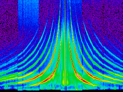
This produces just the bare image "banana.png":
With the S-Lang xfig module, the coordinate system can, however, be easily added (back again).
Plotting the png into an SLxfig plot
It is important to set the correct coordinates for the SLxfig plot object,
as this information is no more present in the bare image.
As discussed above (in the section on "overflow bins"),
the last bins of the reduced 2d-array end where the original grids end
– and obviously the first bins start where the grids start.
This is all the information that needs to be passed to the world method of an SLxfig plot object:
require("xfig");
variable p = xfig_plot_new();
p.world(x_grid[0], x_grid[-1], energy_grid[0]/1000, energy_grid[-1]/1000);  % defining the coordinate system; energy in keV instead of eV
p.plot_png("banana.png");
p.xlabel("Sky X Position");
p.ylabel("Energy [keV]");
p.render("banana-plot.pdf");
The resulting plot looks like this:

