Plot geospatial data (xfig example)
Jump to navigation
Jump to search
Read and use geospatial data
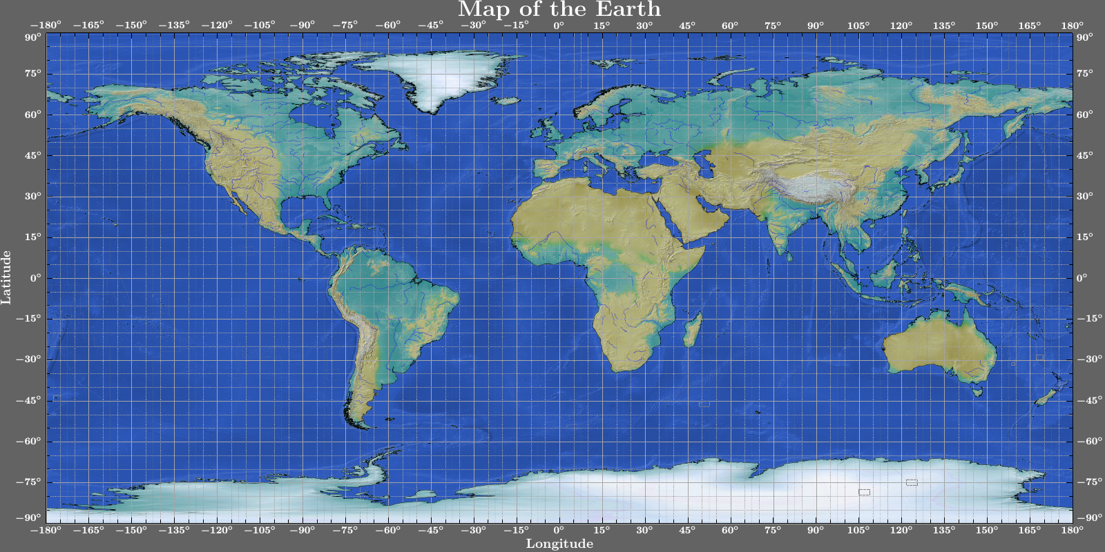
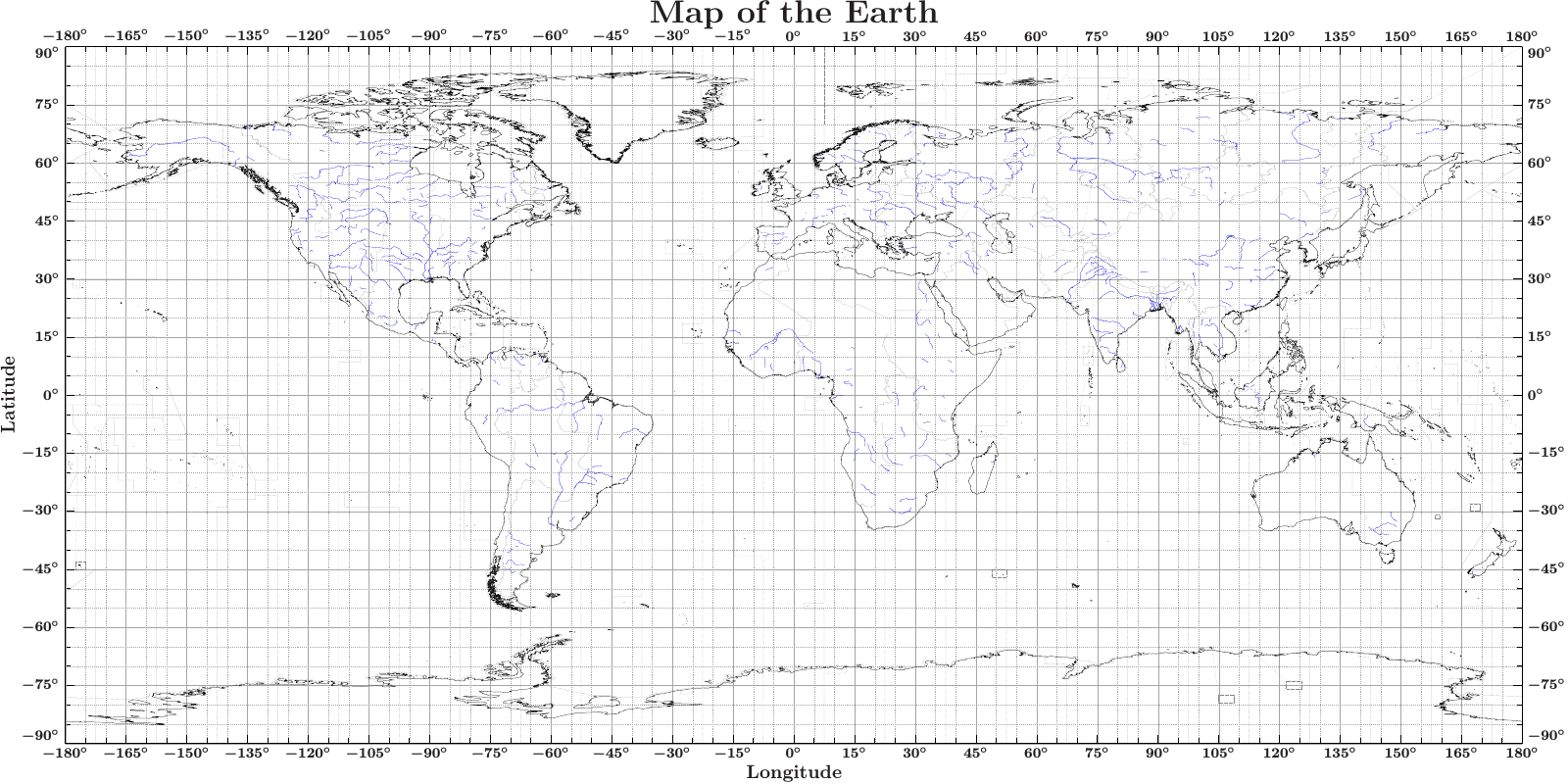
Natural earth provides a huge and free collection of vector and raster data for drawing maps of the earth. Most of the files are distributed as ESRI shape files. Here is demonstrated how you can use the slang wrapper around the shapelib allowing to read this files.
Be aware that the resulting pdf files are huge and are scaled to a physical size of roughly 2 by 1 meter! The images here are only a down sampled version.
The shapelib slang wrapper can be obtained from our git page (internal only). There are numerous bugs, and be prepared to face core dumps when you use it!
require("xfig");
require("shapelib");


% the relevant files for the lines we want to draw
% source is  -- https://www.naturalearthdata.com/ --
% The raster data is taken from the geotiff files and
% converted to simple grayscale png files. All geo data
% is droped and there is no way to get the projection information
% form the WKT (.prj) files! (for me, I have no idea if and how
% this is standardized...)

variable SOURCE = struct {
  coastline = "ne_10m_coastline",
  land = "ne_10m_land",
  islands_coastline = "ne_10m_minor_islands_coastline",
  islands = "ne_10m_minor_islands",
  reefs = "ne_10m_reefs",
  ocean = "ne_10m_ocean",
  rivers = "ne_10m_rivers_lake_centerlines",
  lakes = "ne_10m_lakes",
  grid = struct {
    deg1 = "ne_10m_graticules_1",
    deg5 = "ne_10m_graticules_5",
    deg10 = "ne_10m_graticules_10",
    deg15 = "ne_10m_graticules_15",
    deg20 = "ne_10m_graticules_20",
    deg30 = "ne_10m_graticules_30"
  },
  timezones = "ne_10m_time_zones"
};

variable current_shape;

current_shape = shape_open(SOURCE.coastline, "r");

% lets plot the map in a plot window
variable PLOT = xfig_plot_new(40, 20); % it's to small, but we scale later
PLOT.world(-180,180,-90,90); % that is the coordinates
PLOT.title("Map of the Earth"; size="\\Huge");
PLOT.xlabel("Longitude"; size="\\large");
PLOT.ylabel("Latitude"; size="\\large");
PLOT.xaxis(;major=[-180:180:15], minor=[-180:180:5][where([-180:180:5] mod 15)],
	   format="$%d^\\circ$", major_grid=1, major_line=0, major_width=1, color="#a5a5a5",
	   minor_grid=1, minor_line=1, minor_width=1,
	   ticlabel_size="\\small");
PLOT.yaxis(;major=[-90:90:15], minor=[-90:90:5][where([-90:90:5] mod 15)],
	   format="$%d^\\circ$", major_grid=1, major_line=0, major_width=1, color="#a5a5a5",
	   minor_grid=1, minor_line=1, minor_width=1,
	   ticlabel_size="\\small");

% Define a second plot window so we can have nicer tic marks
variable MARKS = xfig_plot_new(40, 20);
MARKS.world(-180,180,-90,90);
MARKS.xaxis(; major=[-180:180:15], minor=[-180:180:5][where([-180:180:5] mod 15)],
	    ticlabels=0, depth=1, width=3);
MARKS.yaxis(; major=[-90:90:15], minor=[-90:90:5][where([-90:90:5] mod 15)],
	    ticlabels=0, depth=1, width=3);

% the shape struct provides a .next() function to iterate over
% the contents. If we are at the last one it returns null
variable s = current_shape.next();
do {
  PLOT.plot(s.X, s.Y);
  s = current_shape.next();
} while (s != NULL);


% This is commented out, because we use a neat picture to visualize

% Iterate over the land polygons
%current_shape.close(); % close the stuff, we don't want to occupy all that memory
%current_shape = shape_open(SOURCE.land, "r");
%s = current_shape.next();
% The land polygons are a different data type of the shape file, guess what, polygons.
% These are stored as 'parts' in one returned struct. So we have to use the info
% where a part starts (and stops) to draw the correct polygons
variable i, nparts, w;
%do {
%  nparts = length(s.PartStart);
%  _for i (0, nparts-2, 1) {
%    w = [s.PartStart[i]:s.PartStart[i+1]-1];
%    PLOT.shade_region(s.X[w], s.Y[w]; fillcolor="#552525");
%  }
%  w = [s.PartStart[nparts-1]:nparts-1];
%  PLOT.shade_region(s.X[w], s.Y[w]; fillcolor="#552525");
%  s = current_shape.next();
%} while (s != NULL);

% Next on the list is the coastline of the islands
current_shape.close();
current_shape = shape_open(SOURCE.islands_coastline, "r");
s = current_shape.next();
do {
  PLOT.plot(s.X, s.Y); % again ordinary lines, no special treatment necessary
  s = current_shape.next();
} while (s != NULL);

% And also the corresponding land masses
current_shape.close();
current_shape = shape_open(SOURCE.islands, "r");
s = current_shape.next();
do {
  nparts = length(s.PartStart);
  _for i (0, nparts-2, 1) {
    w = [s.PartStart[i]:s.PartsStart[i+1]];
    PLOT.shade_region(s.X[w], s.Y[w]; fillcolor="552525");
  }
  w = [s.PartStart[nparts-1]:nparts-1];
  PLOT.shade_region(s.X[w], s.Y[w]; fillcolor="552525");
  s = current_shape.next();
} while (s != NULL);

% Skip reefs, who needs them, right?
% Go straight to rivers
current_shape.close();
current_shape = shape_open(SOURCE.rivers, "r");
s = current_shape.next();
% These are arcs or polylines, but given as different parts. Sooooo
% same strategy as for the land masses
do {
  nparts = length(s.PartStart);
  if (s.ShapeType == 0) { s = current_shape.next(); continue; } % Type 0 are Null shapes, i.e., have only meta data. skip them
  _for i (0, nparts-2, 1) {
    w = [s.PartStart[i]:s.PartStart[i+1]-1];
    PLOT.plot(s.X[w], s.Y[w]; color="#2525E5");
  }
  w = [s.PartStart[nparts-1]:nparts-1];
  PLOT.plot(s.X[w], s.Y[w]; color="#2525E5");
  s = current_shape.next();
} while (s != NULL);

% Now deal with the lakes, polygons of course
% well, don't they are way to small
%current_shape.close();
%current_shape = shape_open(SOURCE.rivers, "r");
%s = current_shape.next();
%do {
%  nparts = length(s.PartStart);
%  if (s.ShapeType == 0) { s = current_shape.next(); continue; }
%  _for i (0, nparts-2, 1) {
%    w = [s.PartStart[i]:s.PartStart[i+1]-1];
%    PLOT.shade_region(s.X[w], s.Y[w]; fillcolor="#2525E5");
%  }
%  w = [s.PartStart[nparts-1]:nparts-1];
%  PLOT.shade_region(s.X[w], s.Y[w]; fillcolor="#2525E5");
%  s = current_shape.next();
%} while (s != NULL);

% Plot some grid lines
% Well no, we simply use the coordinate grid
%current_shape.close();
%current_shape = shape_open(SOURCE.grid.deg30, "r");
%s = current_shape.next();
%do {
%  PLOT.plot(s.X, s.Y);
%  s = current_shape.next();
%} while (s != NULL);

% Finally get some time zones on the map
current_shape.close();
current_shape = shape_open(SOURCE.timezones, "r");
s = current_shape.next();
do {
  PLOT.plot(s.X, s.Y; line=2, color="#858585");
  s = current_shape.next();
} while (s != NULL);


% For a nice map, use a image. This is also from natural earth, however I manipulated
% some of the resources to get the result.
% GS TAKES FOREVER TO RENDER THIS, comment it out if you want to test the shapelib
%PLOT.plot_png("world.png"; depth=1000);

variable C = xfig_new_compound(PLOT, MARKS);
C.scale(5);
C.render("Map-vector.pdf");

