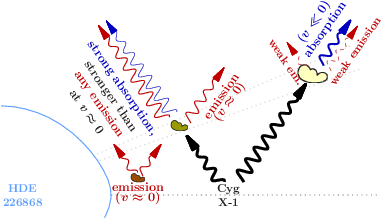
Wind structure of Cyg X-1 (xfig example)

Wind structure of Cyg X-1

The clouds included in this sketch are produced by LaTeX using a package providing weather symbols:

\documentclass{article}
\usepackage{color}
\usepackage[weather]{ifsym}
\begin{document}
\definecolor{c}{rgb}{.6,.3,0}
\pagestyle{empty}
\strut\hbox to 0pt{\color{c}\FilledCloud}\Cloud
\end{document}

Here, a \Cloud is placed ontop of a \FilledCloud (which was put in a horizontal box of zero width) in order to create a contour around the filled cloud.

Processing the resuting postscript file with ps2eps -B recalculates the bounding box and thus produces an eps image containing the cloud only. This step is repeated for three colors c, yielding cloud1.eps, cloud2.eps, and cloud0.eps.

You will also need the Roche lobe contours of the companion star HDE226868. See instructions in Chandra coverage to create them.

When done with the preparations, you can compose the figure:

require("xfig");

xfig_new_color("direct", 0x000000);
xfig_new_color("abs",    0x0000C0);
xfig_new_color("em",     0xC00000);
xfig_new_color("HDE",    0x60A0FF);

% load the Roche lobe contours:
variable t = fits_read_table("Roche_contours_xz_q0.567.fits+2");
struct_filter(t, [::100]);

variable i = 35*PI/180; % inclination of the system
variable factor = 1.15;
variable l = 10/factor/1.1*sin(i), a = .25,  P = .5;

% simplify the use of xfig_new_photon
define add_photon(xfig, x, y)
{
  variable X1, Y1; (X1, Y1) = xfig.xfig_coords(x[0], y[0]);
  variable X2, Y2; (X2, Y2) = xfig.xfig_coords(x[1], y[1]);
  variable ph = xfig_new_photon(vector(X1-X2, Y1-Y2, 0), a, P);
  ph.translate(vector(X2, Y2, 0));
  ph.set_pen_color(qualifier("color", "black"));
  ph.set_fill_color(qualifier("color", "black"));
  ph.set_thickness(qualifier("width", 1));
  ph.set_line_style(qualifier("line", 0));
  xfig.add_object(ph);
}

% setup the plot with a straightforward coordinate system and no axes
variable xfig = xfig_plot_new(20*.8, 21*.8);
xfig.world(0, 2, -.1, 2);
xfig.axes(; off);

% plot the companion star and the binary axis of the system
xfig.plot(t.x, t.z; color="HDE");
xfig.xylabel(0,0,`\centering\small HDE\\226868`, -.5, 0; color="HDE");
xfig.xylabel(1,0,`\centering\small Cyg\\X-1`);
xfig.plot([.48, 1.67], [0, 0]; line=2, color="#808080", width=2);


% Since there will be lots of lines, 
% a couple of linear equations for the coordinates are needed.
% Never mind the horrible coefficients,
% involving the inclination i and user-chosen radii! ;-)

variable r1=.15, R1=.55, rC1=.65;
% x = t * (1-rC1*s^2) = 1+r4 * s^2
% y = t * (s*c*rC1)   = s*c*r4
% => t = r4/rC1
% => r4/rC1 * (1-rC1*s^2) = 1 + r4*s^2
% => r4 * [ (1-rC1*s^2)/rC1 - s^2 ] = 1
variable rC2 = 1/(1/rC1-2*sin(i)^2);
variable R2 = rC2+R1-rC1;
variable r2 = r1;

% some clouds retreat radially from the star, expanding:
variable x = 1-sin(i)^2*rC1;
variable y = sin(i)*cos(i)*rC1;
variable r = hypot(x, y);
variable alpha = atan2(y,x) - .033;
xfig.plot(r*cos(alpha)*[.54, 2], r*sin(alpha)*[.54, 2]; line=2, color="#D0D0D0");
alpha += 2*.033;
xfig.plot(r*cos(alpha)*[.54, 2], r*sin(alpha)*[.54, 2]; line=2, color="#D0D0D0");

% add the clouds:

% load an exisiting .eps file
variable cl = xfig_new_eps("cloud1.eps"); 

% scale it according to your wishes
cl.scale(1.2); 

% and add it as an object to your figure
xfig.add_object(cl, x, y); 

variable cl = xfig_new_eps("cloud2.eps");
cl.set_depth(200);
cl.scale(1.2*hypot(1+sin(i)^2*rC2, sin(i)*cos(i)*rC2)/r);
xfig.add_object(cl, 1+sin(i)^2*rC2, sin(i)*cos(i)*rC2);

x = .6;  y =  .075;
variable cl = xfig_new_eps("cloud0.eps");
cl.scale(1);
xfig.add_object(cl, x, y);

% Since an xfig plot is basically a struct of function references,
% you can easily add your own functions to it:
xfig = struct { @xfig, add_photon=&add_photon };

% Now call add_photon just like any xfig function you already know:
xfig.add_photon(x+[.02,.18]*sin(i),
                y+[.02,.18]*cos(i); color="em", width=2);
xfig.add_photon(x-[.02,.18]*sin(i),
                y+[.02,.18]*cos(i); color="em", width=2);
xfig.xylabel(x, y-0.04, "emission"; color="em");
xfig.xylabel(x, y-0.09, `($v\approx0$)`; color="em");

variable dx = .04;

variable rr1 = rC1*2-R1;
variable RR1 = rr1 + R2-r2;

variable rr2 = rC2*2-R2;
variable RR2 = rr2 + R1-r1;

xfig.add_photon(1-sin(i)^2*[r1-.05,R1], sin(i)*cos(i)*[r1-.05,R1]; color="direct", width=4);
xfig.add_photon(1+sin(i)^2*[r2, R2], sin(i)*cos(i)*[r2, R2]; color="direct", width=4);

xfig.add_photon(1-sin(i)^2*[rr1,RR1],           sin(i)*cos(i)*[rr1,RR1]; color="abs");
xfig.add_photon(1-sin(i)^2*[rr1,RR1]-dx*cos(i), sin(i)*cos(i)*[rr1,RR1]-dx*sin(i); color="em", width=2);
xfig.add_photon(1-sin(i)^2*[rC1,1.5*rC1-.5*RR1]+dx*cos(i),  sin(i)*cos(i)*[rC1,(RR1+rC1)/2]+dx*sin(i); color="em", width=2);

xfig.add_photon(1+sin(i)^2*[rr2,RR2],           sin(i)*cos(i)*[rr2,RR2]; color="abs", width=3);
xfig.add_photon(1+sin(i)^2*[rr2,RR2]+dx*cos(i), sin(i)*cos(i)*[rr2,RR2]-dx*sin(i); color="em", line=1);
xfig.add_photon(1+sin(i)^2*[rC2,1.5*rC2-.5*RR2]-dx*cos(i),  sin(i)*cos(i)*[rC2,(rC2+RR2)/2]+dx*sin(i); color="em", line=1);

% xfig.plot(1+sin(i)^2*[-rC1,rC2], sin(i)*cos(i)*[rC1,rC2]; line=2);

variable r = (rC1+RR1)/2;
variable x = 1-sin(i)^2*r;
variable y = sin(i)*cos(i)*r;
dx = 0.12;
xfig.xylabel(x-    dx*cos(i), y-    dx*sin(i), `strong absorption,`; color="abs", rotate=-55);
xfig.xylabel(x-1.5*dx*cos(i), y-1.5*dx*sin(i), `stronger than`; rotate=-55);
xfig.xylabel(x-2  *dx*cos(i), y-2  *dx*sin(i), `any emission`; color="em", rotate=-55);
xfig.xylabel(x-2.5*dx*cos(i), y-2.5*dx*sin(i), `at $v\approx0$`; rotate=-55);

variable x = 1-sin(i)^2*(1.375*rC1-.375*RR2);
variable y = sin(i)*cos(i)*(rC1+(-.375*rC1+.375*RR1));
variable x = 1-sin(i)^2*(1.375*rC1-.375*RR2);
variable y = sin(i)*cos(i)*(rC1+(-.375*rC1+.375*RR1));
dx /= 1.5;
xfig.xylabel(x+  dx*cos(i), y-  dx*sin(i), `emission`; color="em", rotate=55);
xfig.xylabel(x+1.5*dx*cos(i), y-1.5*dx*sin(i), `($v\approx0$)`; color="em", rotate=55);

variable r = (rC2+2*RR2)/3;
variable x = 1+sin(i)^2*r;
variable y = sin(i)*cos(i)*r;
dx /= 1.25;
xfig.xylabel(x-2  *dx*cos(i), y+2  *dx*sin(i), `($v\ll0$)`; color="abs", rotate=55);
xfig.xylabel(x-    dx*cos(i), y+    dx*sin(i), `absorption`; color="abs", rotate=55);
xfig.xylabel(x+1.5*dx*cos(i), y-1.5*dx*sin(i), `\small weak emission`; color="em", rotate=55);

dx *= 1.25;
xfig.xylabel(1+sin(i)^2*(1.5*rC2-.5*RR2)-dx*sin(i),  sin(i)*cos(i)*(rC2+RR2)/2-dx*cos(i),
             `\small weak em.`; color="em", rotate=-55, depth=10);

xfig.render("sketch.eps");