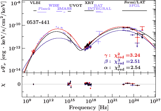
Plot fit model (xfig example)

Note: This only contains parts of the original script, showing how to plot the fit model.

%For a Plot with Hz as x-axis
% for keV axis use built-in function eval_fun_keV

require("isisscripts");
variable plan=4.135667516e-18; %Planck constant
define eval_fun_hz(hz_bin_lo, hz_bin_hi)
{  
    variable A_bin_lo = _A(hz_bin_hi*plan);
    variable A_bin_hi = _A(hz_bin_lo*plan);
    variable flux = eval_fun(A_bin_lo, A_bin_hi);
    return reverse(flux);  
}  


%Load model
load_par("best_fit.par");

%Get unassorbed/dereddened model
%Chose whatever model or component you want to show

fit_fun("(logpar(1)+logpar(2)+zbbody(1))");


%Get the x grid where you want to evaluate your model
variable lo,hi;

(lo, hi) = log_grid (1e9, 1e26, 5000);

%Evaluate model on the defined grid
variable a = eval_fun_hz(lo,hi);
%Note: Output is in bin-integrated photon flux: ph/s/cm^2/bin

variable k = 1./624150636.3094;  %keV2ergs

%Conversion to differential energy flux (assuming constant flux in bin): erg/s/cm^2
variable conv_factor = (0.5 * ((lo*plan) + (hi*plan)))^2/((hi*plan)-
(lo*plan))*k;

%Apply flux conversion to model
variable model = conv_factor*a;

%For log plotting: set 0 values to very small ones
model[where (model==0)]=1e-29;


%In an initialized xfig plot:
%Note: linear center of bin not log, because grid is fine enough
pl.plot((lo+hi)/2., model;color="black",width=2,depth=50);