GX304batlcobs (xfig example)
Jump to navigation
Jump to search
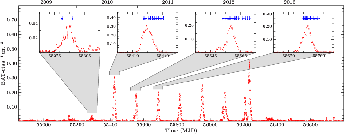
Insets as zoom-ins

require("isisscripts");

%%% all necessary data

% get ObsIDs, tstart, and tstop of all used data from somewhere
variable data = struct {
  obsid = [...],
  tstart = [...],
  tstop = [...]
}

% load BAT-lightcurve
variable bat = fits_read_table("source.lc.fits");

%%% initialize xfig plot

variable W = 28, H = 10; % width and height of the full-lc plot
variable wt0 = 54850, wt1 = 56800; % xrange in MJD of this plot
variable Wi = 5.2, Hi = 3.5; % width and height of the zoom plots
variable pl = xfig_plot_new(W,H);
% set world; the negative, small pad-values removes the tic-labels
% at the end of each axis (my personal liking)
pl.world(wt0, wt1, 0, 0.8; padx = -1e-6, pady = -1e-6);
% set 2nd world, here the years
pl.world2(yearOfMJD(pl.get_world()[0]), yearOfMJD(pl.get_world()[1]),
	  __push_array(pl.get_world()[[2,3]]); padx = -1e-6, pady = -1e-6);
pl.x2axis(; major = [2009:2014]+.5-1e-6, minor = [2009:2015],
            major_len = 0, minor_len = .2, format= " %.0f");
pl.y2axis(; ticlabels = 0);
pl.y1axis(; format = "%.2f");
pl.xlabel("Time (MJD)");
pl.ylabel("BAT-cts\,s$^{-1}$\,cm$^{-2}$"R);

%%% plot lightcurve

pl.plot(bat.time, bat.rate, bat.error; color = "red", sym = "x",
        width = 1, size = .5);

%%% create zoom plots

variable pli = Struct_Type[4]; % an array of structures; for each plot one element
variable t0 = [55260, 55395, 55520, 55655]; % the start (in MJD) for each plot
variable dt = 60; % the length (in days) for every plot (such that the scaling is equal for all)
variable ymx = [0.05, 0.42, 0.27, 0.28]; % the maximum y-value for each plot (in cts/s/cm^2)
variable dx = .24; % the relative spacing between each plot (measured from their centers)

% loop over all plots and create them
variable i;
_for i (0, length(pli)-1, 1) {
  %%% initialize the zoom plots
  pli[i] = xfig_plot_new(Wi, Hi);
  pli[i].world(t0[i], t0[i]+dt, 0, ymx[i]*1.1; pady = -1e-6);
  pli[i].xaxis(; major = t0[i]+[.25,.75]*dt, minor = t0[i]+[0:dt:10],
                 ticlabel_size = "footnotesize");
  pli[i].y1axis(; ticlabel_size = "footnotesize", format = "%.2f");
  pli[i].x2axis(; ticlabels = 0);

  %%% plot the lightcurve
  pli[i].plot(bat.time, bat.rate, bat.error; color = "red", sym = "x",
              width = 1, size = .5);
  % add the observation times
  pli[i].plot(.5*(data.tstart+data.tstop), ones(length(data.tstart))*ymx[i];
              sym = "darr", color = "blue");

  %%% add the object to the full lightcurve plot
  variable ix = .5*(1.-dx*length(pli)) + dx*(i+.5); % relative x-coordinate of the zoom plot
  pl.add_object(pli[i], ix, .55, 0, -.5; world0);

  %%% calculate the xy-positions for the lines connecting
  %%% the zoom plots with the full lightcurve

  % relative x/y-coordinates of the lower-[left,right]-corner of the zoom plot
  variable xi = (pli[i].plot_data.X.x + [0, Wi]) / W;
  variable yi = pli[i].plot_data.X[0].y / H * [1,1];
  % relative x/y-coordinates of the [beginning,end] of the zoom time range _in_ the full lightcurve plot
  variable xl = 1.*(t0[i]+[0,dt]-wt0) / (wt1-wt0);
  variable yl = (max(bat.rate[where(t0[i] < bat.time < t0[i]+dt)]) + [0.02, 0.04]) / .8;

  %%% plot the connecting lines
  pl.plot([xl[0], xl[0], xi[0]], [yl, yi[0]]; world0, color = "gray");
  pl.plot([xl[1], xl[1], xi[1]], [yl, yi[1]]; world0, color = "gray");
  % shade the area in between
  pl.shade_region(
    [xl[0], xl[0], xi[0], xi[1], xl[1], xl[1], xl[1]],
    [yl[0], yl[1], yi[0], yi[1], yl[1], yl[0], yl[0]];
    color = "#DDDDDD", world0
  );
}

% render
pl.render("BAT_lc.pdf");