Timing tools
Foucalc
[In work! You might use it as a reference in the meantime, but some things are not yet covered. Also let me know if things are not clear! - VG]
The basic tool for X-ray timing analysis with the Remeis scripts is foucalc [1], which calculates power-, cross power-, coherence- and timelag-spectra [2]. It requires equally spaced, gapless lightcurves as well as the length of the lightcurve segment on which the Fourier transformation is to be performed, given in number of bins. Note that because the underlying algorithm is FFT, the segment length should be a power of two to increase the performance.
When only one lightcurve is given, foucalc calculates the power density and related quantities only. When more than one lightcurve is given, the cross power-, coherence- and timelag-spectra are calculated for all pairs of lightcurves. The lightcurves have to be in the format:
lc = struct { time=[t_1, t_2, ...], rate1=[r1_1, r1_2, ...], rate2=..., rate3= };
The time has to be given in seconds (so be cautious when using fits_read_lc, which usually returns the time in MJD).
If you use RXTE/PCA lightcurves, don't forget to set the numinst keyword, which defines the number of instruments (=PCUs) on, since otherwise your noise correction will be wrong. If you are not using RXTE/PCA set the deadtime keyword to whatever is appropriate for the instrument you are using (e.g. 0).
Given a single PSD value before any further calculations, its uncertainty will be of the same order of magnitude as the PSD itself. Averaging therefore crucial. This is build in into foucalc: given a lightcurve of say 1288192 bins and a segment length of 16384, foucalc will calculate a PSDs on every segment and average every value over all 1288192/15385 = 78 segments.
PSDs
Calculating the PSD
Given two PCA lightcurves,
50110-01-45-00_437_AND_good_14off_excl_0-10.lc
and
50110-01-45-00_437_AND_good_14off_excl_11-13.lc
(which have been checked for gaps and found to be gapless [3] ) we want to calculate and bin the PSD, lags and coherence.
%% read in lightcurves
variable lc1 = fits_read_table("50110-01-45-00_438_AND_good_14off_excl_0-10.lc");
variable lc2 = fits_read_table("50110-01-45-00_438_AND_good_14off_excl_11-13.lc");

%%define variables to store average rate of lightcurve & rms
variable rms,avg;

%%calculate timing quantities
variable result = foucalc(struct{time=lc1.time,rate1=lc1.rate,rate2=lc2.rate},16384;
                          numinst=3,RMS=&rms,avgrate=&avg,verbose);
This produces the following output - thank to the verbose keyword:
light curves: 2516 s with 1288192 bins of 0.00195312 s  (0 s gaps)
  segmentation: 78 segments of 16384 bins
=> frequencies: 0.03125-256 Hz.
Power spectra will be calculated in Miyamoto-normalization.
Calculating power spectrum for rate1.  RMS(0.03125-256 Hz) = 27.1%
Calculating power spectrum for rate2.  RMS(0.03125-256 Hz) = 25.7%
Calculating cross power spectrum (=> coherence and timelags) for rate1 and rate2.
This is right now the only place at which foucalc will complain if the lightcurve contains gap. It will calculate the quantities even if the lightcurve contains gaps - only you can't trust your results. Therefore: use verbose, check that you've done everything right, at least while building up your scripts.
Plot the PSD for the first lightcurve with:
xlog;ylog;plot_with_err(result.freq,result.signormpsd1,result.errnormpsd1);
Rebinning the PSD
The uncertainties on the individual PSDs values are still large, especially at high frequencies. To further improve the SNR, the PSD is rebinned to a new frequency grid and the final PSDs is then the average over the individual PSDs at the frequencies corresponding to the frequencies included into the new frequency bin. Mostly, a logarithmic rebinning with df/f = const. is used, a typical value would be df/f = 0.15 .
Quantities calculated with foucalc are rebinned with the rebin_fouquan tool - the quantity and it's error have to be rebinned in two individual steps:
variable reb_psd = rebin_fouquan(result.freq,result.signormpsd1,
                                 result.numavgall;logfreq=0.15);
variable reb_err = rebin_fouquan(result.freq,result.errnormpsd1,
                                 result.numavgall;logfreq=0.15);
reb_err does not yet contain the real errors of the psds, but needs to be weighted with the square root of the number of values the averaging was performed over. The final PSD is therefore:
variable psd1 = struct{freq_lo = reb_psd.freq_lo,freq_hi=reb_psd.freq_hi,
  value = reb_psd.value, error= reb_err.value/sqrt(reb_err.n)};
Once again plot you PSD - either as PSD vs. frequency or PSD x frequency vs. frequency:
%%PSD vs. frequency
xlog;ylog;plot_with_err((psd1.freq_lo+psd1.freq_hi)/2,psd1.value,psd1.error);

%%PSDxfreuency vs. frequency
xlog;ylog;plot_with_err((psd1.freq_lo+psd1.freq_hi)/2, psd1.value*(psd1.freq_lo+psd1.freq_hi)/2,
psd1.error*(psd1.freq_lo+psd1.freq_hi)/2);
Lag-energy spectrum for archival XMM-Newton data
[--- under construction --- written by OK, please ask if something is unclear!; last edit by AG (10 Aug 2020) regarding the correction of telemetry drop-outs]
The following is an example how to compute PSDs, a lag-frequency spectrum, and a lag-energy spectrum on archival XMM-Newton data of GX 339-4 [4].
We start by extracting the XMM-Newton PN lightcurve in two energy bands (500-900eV and 2000-3000eV)
#!/bin/tcsh
source $SOFTDIR/sas_init.csh # initialize the SAS software
set xmmscripts=${XMMTOOLS} # make sure the proper xmmscripts are loaded
set obsid='0204730201'
set datadir=/userdata/data/koenig/GX339-4/XMM-2004-03-16/odf
set dt=0.1

${xmmscripts}/xmmprepare --datadir=$datadir --prepdir=$obsid --pn --noapplyflaregti --timing --notimelog # prepare the data

${xmmscripts}/xmmextract --prepdir=$obsid --pn --timing --full --energyband="500,900" --noflarescreen --defaultpattern --dt=$dt --clobber
${xmmscripts}/xmmextract --prepdir=$obsid --pn --timing --full --energyband="2000,3000" --noflarescreen --defaultpattern --dt=$dt --clobber
Now we can start the analysis. Let's load the data and the Good Time Intervals (GTI) information to be able to correct the light curve for the telemetry drop-outs:
require("isisscripts");

%% Load the lightcurve and GTI file
a=fits_read_table("full_sd_0.1s_0500-0900.lc");
b=fits_read_table("full_sd_0.1s_2000-3000.lc");
gtia=fits_read_table("full_sd_0.1s_0500-0900.lc[GTI00006]");
gtib=fits_read_table("full_sd_0.1s_2000-3000.lc[GTI00006]");

%% Get the start time such that LC starts at 0s
tstart=fits_read_key("full_sd_0.1s_0500-0900.lc[1]", "TSTART");
The time information in the light curve is not given as a grid, however, a time grid with connecting high to low bins is necessary for the filter_gti function to filter out all time bins with an unsufficient fractional exposure. Compared to the default binning width of 100s, telemetry drop-outs can last for only a few seconds, hence only datapoints with times values that fall directly in the gaps between the GTIs, are sorted out. This can be avoided by inserting a grid, which we have to create from the information in the light curve FITS-file. Something that might be important for some analyses is the information about at which position in the grid the given time data points have to be set (either beginning, middle or the end). This is instrument dependent, and should be usually found either in the header or the manual.
%% The binning width is encoded in the header with the keyword TIMEDEL
variable tdiff = fits_read_key("full_sd_0.1s_0500-0900.lc[1]", "TIMEDEL");
variable trel = 0.5;

variable tlo_a = a.time - trel*tdiff;
variable thi_a = a.time + (1.-trel)*tdiff;
variable tlo_b = b.time - trel*tdiff;
variable thi_b = b.time + (1.-trel)*tdiff;
Now we can go ahead and correct the light curve. As the default value of the fractional exposure (fracexp) is set to a very low limit, one needs to set this to a reasonable high level (e.g. 90-95%). We can insert this information via the corresponding qualifier.
%% Subtract TSTART and do GTI correction
variable minimum_frac = 0.95;
(filta,filtb)     = filter_gti(tlo_a, thi_a, gtia; minfracexp=minimum_frac), filter_gti(tlo_b, thi_b ,gtib; minfracexp=minimum_frac);
(timea,timeb)     = a.time[filta]-tstart,b.time[filtb]-tstart;
(countsa,countsb) = a.counts[filta],b.counts[filtb];
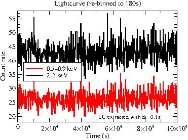
If we plot the (re-binned) lightcurve, there is not much to see.
Fortunately, we can do a Fourier analysis in order to reveal the variability and correlations of these lightcurves. As described above, this can be done with the foucalc routine. I choose the Miyamoto normalization (see [5]) as in the publication. This normalization yields the PSD in units of fractional root mean square (rms/Rsignal)2.
%% Choose segment length
dimseg=8192; % (bins), should be a power of 2 for FFT
dt=0.1; % (s), timing resolution of lightcurve extraction

%% Compute PSDs, CPD, and time lags with foucalc
r=foucalc( struct{time=timea, rate1=countsa/dt, rate2=countsb/dt}, dimseg ; normtype="Miyamoto");
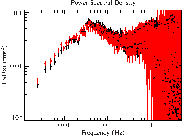
xlog;plot_with_err(r.freq,r.signormpsd1*r.freq,r.errnormpsd1*r.freq);

%% There is a warning that there are gaps in the LC (due to the telemetry dropouts) if verbose is set in foucalc. We ignore that for this simple analysis.
File:Gx399m4 xmm psd unbinned.pdf
This really needs some re-binning to increase the S/N-ratio. All foucalc quantities can be re-binned with the rebin_fouquan routine (note that the PSD has already been binned when we set the length of the segments.).
%% Choose Delta f/f, the logarithmic frequency resolution
dff=0.15;
reb_psd1 = rebin_fouquan(r.freq, r.signormpsd1, r.numavgall ; logfreq=dff);
reb_err1 = rebin_fouquan(r.freq, r.errnormpsd1, r.numavgall ; logfreq=dff);
reb_psd2 = rebin_fouquan(r.freq, r.signormpsd2, r.numavgall ; logfreq=dff);
reb_err2 = rebin_fouquan(r.freq, r.errnormpsd2, r.numavgall ; logfreq=dff);

%% Need to weight the PSD error with the square root of the number of values the averaging was performed over
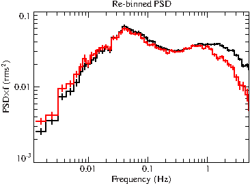
ylog;hplot_with_err( reb_psd1.freq_lo, reb_psd1.freq_hi, reb_psd1.value*reb_psd1.freq_lo, reb_err1.value/sqrt(reb_err1.n)*reb_psd1.freq_lo );
File:Gx339m4 xmm psd binned.pdf
What can we deduce from this PSD? We observe that the minimum sampled frequency is 1/dimseg - if you choose a long segment length, small quantities can be sampled but then also the S/N-ratio is smaller. On the other hand, choosing a small segment length can lead to an effect called red-noise leakage, which is due to the finite extend of the data (also called windowing, see [6] p.8ff or [7] p.14f.). The maximum sampled frequency is 1/(2*dt), where dt is the timing resolution of the lightcurve. This is called the Nyquist frequency.
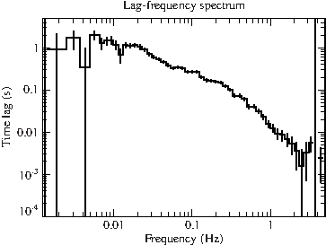
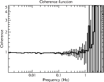
foucalc also computes the time lag between the two lightcurves. Let's first rebin and then plot them together with the coherence:
For the curious:
The time-lag is computed from the phase of the cross-power density. The CPD is a complex quantity and thus has an imaginary and real part (see, e.g., Uttley+14 eq.8-10): C~eiφ=cos(φ)+isin(φ) => φ=arctan(Im/Re) with the time lag τ=φ/(2πf). In code phase=atan2(r.imagcpd12,r.realcpd12); tlag = phase/(2*PI*r.freq);.
%% Rebin time lag results
reb_lag12 = rebin_fouquan(r.freq, r.lag12, r.numavgall ; logfreq=dff);
reb_errlag12 = rebin_fouquan(r.freq, r.errlag12, r.numavgall ; logfreq=dff);
hplot_with_err(reb_lag12.freq_lo, reb_lag12.freq_hi, reb_lag12.value, reb_errlag12.value/sqrt(reb_errlag12.n) );

%% Rebin coherence function
reb_cof12 = rebin_fouquan(r.freq, r.cof12, r.numavgall ; logfreq=dff);
reb_errcof12 = rebin_fouquan(r.freq, r.errcof12, r.numavgall ; logfreq=dff);
hplot_with_err( reb_cof12.freq_lo, reb_cof12.freq_hi, reb_cof12.value, reb_errcof12.value/sqrt(reb_errcof12.n) );
File:Gx339m4 xmm tlag.pdf File:Gx339m4 xmm coherence.pdf
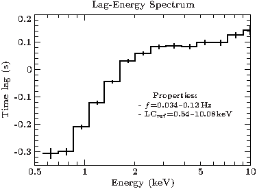
The coherence function is 1 at low frequencies showing a perfect (linear) correlation of the two lightcurves (values above 1 are possible due to counting noise, see Sect. 3.4.1 and 3.5.3 in Katja's diss.). As a final step, we calculate the lag-energy spectrum, by extracting lightcurves in logarithmically binned energy intervals, and calculating their timelags.
refeband=[540,10080]; % (eV), lower and upper bound of energy reference band
reffreqband=[0.034,0.12]; %% (Hz), lower and upper bound of frequency reference band, as in Fig. 2(a) of Uttley+11

fnameref=sprintf("%sfull_sd_0.1s_%04d-%d.lc",datadir,refeband[0],refeband[1]);
lcref       = fits_read_table(fnameref);
lcrefgti    = fits_read_table(fnameref+"[GTI00006]"); % GTI correction
filtref     = filter_gti(lcref.time, lcrefgti);
timelcref   = lcref.time[filtref]-tstart;
cratelcref = lcref.counts[filtref]/dt;

(elo,ehi)=log_grid(500,10000,14); % define logarithmic energy bins

tlags=Double_Type[length(elo)];
tlagerrs=Double_Type[length(elo)];

_for ii (0,length(elo)-1,1) {
  lcname=sprintf("full_sd_0.1s_%04.0f-%04.0f.lc",elo[ii],ehi[ii]);
  if (ehi[ii]>9999) { lcname=sprintf("full_sd_0.1s_%04.0f-%05.0f.lc",elo[ii],ehi[ii]); };

  lc = fits_read_table(lcname);
  lcgti = fits_read_table(lcname+"[GTI00006]");
  filtgti = filter_gti(lc.time, lcgti);

  timelc=lc.time[filtgti]-tstart; %% Do GTI correction
  cratelc=lc.counts[filtgti]/dt;

  %% Calculate PSD, cross-spectrum (CPD) and lags with foucalc
  %% Note that we subtract off the small band LC from the reference
  %% LC. Uttley+11 call this a Channel-of-interest (CI) correction.
  %% This is needed to account for the Poisson noise which is
  %% correlated for both LCs. See also Uttley+11 Sect 3.2.
  r=foucalc(struct{time=timelcref, rate1=cratelcref-cratelc, rate2=cratelc}, dimseg ; normtype="Miyamoto");

  %% Filter the CPD / timelag array for the given frequency range
  filt=where(reffreqband[0]<=r.freq<=reffreqband[1]);

  %% Compute average time lag as arithmetic weighted mean
  tlags[ii]=weighted_mean(r.lag12[filt] ; err=r.errlag12[filt]);
  tlagerrs[ii]=1./sqrt(sum(1/r.errlag12[filt]^2));
}

ylin;hplot_with_err(elo/1000., ehi/1000., tlags, tlagerrs);
File:Gx339m4 xmm lagenergy.pdf
References
- ↑ The original version of the Remeis timing scripts were written by Katja Pottschmidt. When using the tools, please cite Pottschmidt et al. 2003, A&A 407, 1039 and Pottschmidt et al. 2000, A&A 357, L17; see also Nowak et al., 1999, ApJ 510, 874
- ↑ What these are is wonderfully explained in Katja Pottschmidt's PhD Thesis
- ↑ A useful function for this is split_lc_at_gaps
- ↑ The corresponding publication is Uttley, P. e al, MNRAS, Vol. 414, I. 1, pp. L60-L64 (2011)
- ↑ Miyamoto et al., ApJ, 391:L21-L24 (1992) or Katja's dissertation,p.68f
- ↑ M. van der Klies 1988
- ↑ Uttley, P. et al., A&A Review, Volume 22, article id.72, 66 pp., 2014
