Difference between revisions of "Pulse Profiles: A quickstart guide"
Thalhammer (talk | contribs) m |
Thalhammer (talk | contribs) |
||
| (2 intermediate revisions by the same user not shown) | |||
| Line 4: | Line 4: | ||
This is a very short introduction on how to generate X-ray pulse profile in ISIS. To begin, you need either the arrival times of all the events in your observation or a light-curve of this observation. While it is less important when using a local pulse period and a short observation, it would be advisable to use barycentered times and depending on your source apply also orbital correction (usually less important). | This is a very short introduction on how to generate X-ray pulse profile in ISIS. To begin, you need either the arrival times of all the events in your observation or a light-curve of this observation. While it is less important when using a local pulse period and a short observation, it would be advisable to use barycentered times and depending on your source apply also orbital correction (usually less important). | ||
| − | In the following we will use a NICER observation of EXO 2030 | + | In the following we will use a NICER observation of EXO 2030+375 as an example. |
| Line 12: | Line 12: | ||
EN / 1keV = PI * 0.01 . | EN / 1keV = PI * 0.01 . | ||
For NuSTAR the relation would be | For NuSTAR the relation would be | ||
| − | EN / 1keV | + | EN / 1keV = PI * 0.04 + 1.6 . |
<pre> | <pre> | ||
| Line 23: | Line 23: | ||
</pre> | </pre> | ||
| − | To find the local pulse period we use the function "epfold" (make sure to consult | + | To find the local pulse period we use the function "epfold" (make sure to consult 'help epfold') to fold the event times onto a range of trial pulse periods and calculate according to some statistic where the resulting profile shows the most deviation from flat noise. |
It is crucial for both speed and accuracy of this step to provide a reasonable range of periods. | It is crucial for both speed and accuracy of this step to provide a reasonable range of periods. | ||
Further you want to provide the GTIs where events were actually detectable. | Further you want to provide the GTIs where events were actually detectable. | ||
| Line 42: | Line 42: | ||
</pre> | </pre> | ||
| − | [[file:Epfold.png]] | + | [[file:Epfold.png|560px]] |
| − | Finding the peak of this function can also be made more precise, e.g. by fitting a Gaussian, but will keep it simple in this example. Now that we know the local period, we can simply fold on this period to get profile. Consult "help pfold" if you want e.g. a higher number of phase bins: | + | Finding the peak of this function can also be made more precise, e.g. by fitting a Gaussian, but we will keep it simple in this example. Now that we know the local period, we can simply fold on this period to get profile. Consult "help pfold" if you want e.g. a higher number of phase bins: |
<pre> | <pre> | ||
| Line 51: | Line 51: | ||
</pre> | </pre> | ||
| − | [[file:Pprofile.png]] | + | [[file:Pprofile.png|560px]] |
| − | |||
=== Pulse profiles from light-curves === | === Pulse profiles from light-curves === | ||
| − | The whole thing can also be done using light-curves. The advantage is that this includes for some observatories, e.g. NuSTAR, | + | The whole thing can also be done using light-curves. The advantage is that this includes for some observatories, e.g. NuSTAR, additional corrections such as vignetting. Further this allows for background to be subtracted. However, each energy selection requires a new run of e.g nuextract. The script would then look like this: |
| Line 73: | Line 72: | ||
=== Further resources: === | === Further resources: === | ||
| − | * It might be interesting to read up on | + | * It might be interesting to read up on some of the higher level functions implemented by Matthias: find_peak, pulseperiod_search, pulseperiod_magic, pulseperiod_epfold |
| − | * There is also a pulse profile review in work. A draft of which can be | + | * There is also a pulse profile review in work. A draft of which can be obtained e.g. by asking Joern. |
| − | |||
[[Category:Isis / Slang]] | [[Category:Isis / Slang]] | ||
Latest revision as of 17:00, 7 June 2024
Pulse Profiles in ISIS
This is a very short introduction on how to generate X-ray pulse profile in ISIS. To begin, you need either the arrival times of all the events in your observation or a light-curve of this observation. While it is less important when using a local pulse period and a short observation, it would be advisable to use barycentered times and depending on your source apply also orbital correction (usually less important).
In the following we will use a NICER observation of EXO 2030+375 as an example.
Pulse profiles from event files
First we want to describe the generation of pulse profiles directly from the (cleaned) event file. For this we load the event file into ISIS. Then we might want to select the events by their energy, which is usually quantified in the PI or PHA parameter in the eventfile. For NICER the relationship is simply
EN / 1keV = PI * 0.01 .
For NuSTAR the relation would be
EN / 1keV = PI * 0.04 + 1.6 .
variable filename = "/userdata/data/thalhammer/3C50_EXO230_highres/4201960150/ni4201960150_0mpu7_cl.evt";

variable evts = fits_read_table(filename);

variable n = where (50 < evts.pi < 1000 );
variable tms = evts.time [n] ;
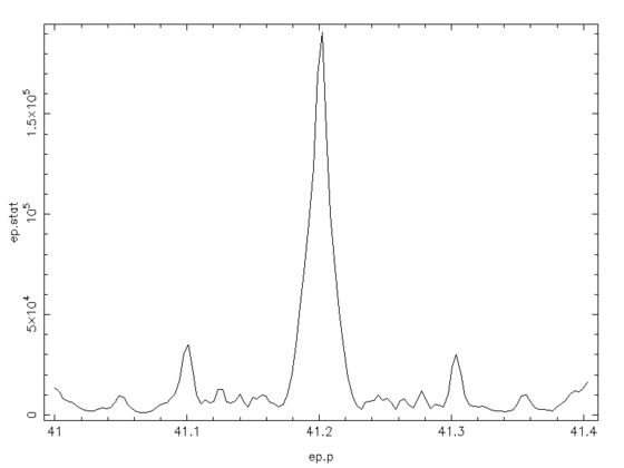
To find the local pulse period we use the function "epfold" (make sure to consult 'help epfold') to fold the event times onto a range of trial pulse periods and calculate according to some statistic where the resulting profile shows the most deviation from flat noise. It is crucial for both speed and accuracy of this step to provide a reasonable range of periods. Further you want to provide the GTIs where events were actually detectable.
variable gti = fits_read_table( filename + "[GTI]");

variable ep = epfold(tms,41.15,41.25;gti=gti);
To find the local period we will first have a look at the resulting statistic and determine its maximum. You know that your results are reliable if the plot below "looks like its giving you the finger" and has a clear maximum:
xlabel("ep.p"); ylabel("ep.stat");
plot(ep.p , ep.stat);

variable p = ep.p [wherefirstmax (ep.stat)];
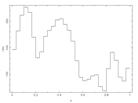
Finding the peak of this function can also be made more precise, e.g. by fitting a Gaussian, but we will keep it simple in this example. Now that we know the local period, we can simply fold on this period to get profile. Consult "help pfold" if you want e.g. a higher number of phase bins:
variable pf = pfold(tms, p ;gti=gti);
hplot_with_err (pf);
Pulse profiles from light-curves
The whole thing can also be done using light-curves. The advantage is that this includes for some observatories, e.g. NuSTAR, additional corrections such as vignetting. Further this allows for background to be subtracted. However, each energy selection requires a new run of e.g nuextract. The script would then look like this:
variable filename = "ni4201960150_0.01s_0500eV-10000eV.lc";
variable dt = 0.01;
variable lc = fits_read_table(filename);
variable gti = fits_read_table(filename+"[GTI]");

variable ep = epfold(lc.time,lc.rate,41.0,41.4;gti=gti ,dt=dt*lc.fracexp);
variable p = ep.p [wherefirstmax (ep.stat)];

variable pf = pfold(lc.time,lc.rate, p;dt=dt,gti=gti,fracexp=lc.fracexp);
Further resources:
- It might be interesting to read up on some of the higher level functions implemented by Matthias: find_peak, pulseperiod_search, pulseperiod_magic, pulseperiod_epfold
- There is also a pulse profile review in work. A draft of which can be obtained e.g. by asking Joern.

