Difference between revisions of "Making tables with sltable"
Thalhammer (talk | contribs) (Fixed typo) |
Thalhammer (talk | contribs) (Fixed Images) |
||
| Line 104: | Line 104: | ||
which, when dropped into a proper LaTeX document, results in the following table: | which, when dropped into a proper LaTeX document, results in the following table: | ||
| − | + | [[File:very_simple_table.png|200px]] | |
This is not a particularly fancy-looking table, but it gets the essential bits: numbers, in the right places, with error bars, and some sort of indication when a parameter is frozen. | This is not a particularly fancy-looking table, but it gets the essential bits: numbers, in the right places, with error bars, and some sort of indication when a parameter is frozen. | ||
| Line 149: | Line 149: | ||
which looks like this once compiled: | which looks like this once compiled: | ||
| − | + | [[File:sltable_simple_table.png|400px]] | |
Much nicer! | Much nicer! | ||
| Line 281: | Line 281: | ||
The table, once compiled with LaTeX, looks like this: | The table, once compiled with LaTeX, looks like this: | ||
| − | + | [[File:sltable_multi_obs_table.png|650px]] | |
For a good time, try adding the qualifiers "horiz=1,landscape=1" and swapping the "rownames" and "colnames" qualifiers. You should get something like this: | For a good time, try adding the qualifiers "horiz=1,landscape=1" and swapping the "rownames" and "colnames" qualifiers. You should get something like this: | ||
| − | + | ||
| + | [[File:sltable_multi_obs_table_horiz.png|1050px]] | ||
There is one issue, which is that the footnote should be accompanied by a marker on the iron line area (i.e., <tt>A_Fe</tt> should have an asterisk next to it). I haven't figured out a sensible way to approach this, so right now you'll have to add those in by hand. | There is one issue, which is that the footnote should be accompanied by a marker on the iron line area (i.e., <tt>A_Fe</tt> should have an asterisk next to it). I haven't figured out a sensible way to approach this, so right now you'll have to add those in by hand. | ||
Revision as of 13:53, 10 July 2018
sltable() is a function designed to streamline the production of LaTeX tables from ISIS data structures. It's put together with the intent of being able to go from a single call to get_params() to a functional LaTeX table in as few steps as possible.
The following examples all start from files saved with the save_par() function, but note that sltable() does not require that you start from here: as explained in the documentation, sltable() is perfectly happy to work with arrays of numbers or strings, or any struct with a "value" field. The function is thus not limited to spectral fits, although spectral fits are what were in mind when it was written.
The basic structure of a call to sltable() is
table = sltable(par1, par2, ...; <qualifiers>);
Each argument given to sltable() is interpreted as one column of the table (or one row if the "horiz" qualifier is nonzero). The arguments can be arrays of strings, which will be printed as-is, arrays of numbers, which will be rounded to three sig figs, or structs. Structs should be of the form:
struct{value,min,max,freeze,limit,nodata}
Only the "value" field is strictly needed; "min" and "max" fields will be used to determine and format error bars, the "freeze" field can be used to specify when a value is frozen, and a "limit" field can be used to indicate whether a value's uncertainties reaching zero is "important" or not (e.g., a power-law's normalization should have "limit=1" set, a power-law's photon index should not). The "nodata" field will cause a \nodata symbol to be printed (or whatever you specify in the "nodata" qualifier in your call to sltable()). This is useful if you want to, e.g., have different models in the same table.
Structs can be provided either as an array of structs (as returned by, e.g., get_params()) or a struct with arrays for its fields. That is, the following two commands produce the same output:
isis> t1 = sltable(struct{value=[1,2,3]});
isis> t2 = sltable([struct{value=1},struct{value=2},struct{value=3}]);
isis> t1 == t2 ? print("Tables match!") : print("tables don't match");
"Tables match!"
<pre>
Note that <code>sltable([1,2,3])</code> also produces the same output as the above two commands. However, with structs you can do much fancier things. Consider:
<pre>
isis> sltable([struct{value=1},struct{value="foo"}],[struct{value="bar"},struct{value=3,min=2,max=4}]);
\begin{deluxetable}{lr}
  \tabletypesize{\footnotesize}
  \tablewidth{0pt}
  \tablecaption{\label{placeholder}}
  \tablehead{}
  \startdata
    $1.00$ & bar \\
    foo & $3.0\pm1.0$ \\
  \enddata
\end{deluxetable}
Since arrays of structs don't need their "value" fields to have the same type - and indeed can have different fields present entirely - we can have different datatypes in different cells, some values, some text, some values with uncertainties.
Next, I'll give a set of more practical examples.
A simple example: Just the numbers
Say you have a set of best-fit parameters saved in the file best.err, with error bars found via, e.g., conf_loop() and saved with save_par(). The file looks like this:
tbnew_feo(1)*(enflux(1,powerlaw(1)*highecut(1))+gaussian(1)+gaussian(2))
 idx  param              tie-to  freeze         value         min         max
  1  tbnew_feo(1).nH         0     0         0.513343           0    4.444283  10^22
  2  tbnew_feo(1).O          0     1                1           0           5
  3  tbnew_feo(1).Fe         0     1                1           0           5
  4  tbnew_feo(1).redshift   0     1                0           0          10
  5  powerlaw(1).norm        0     1                1           0       1e+10
  6  powerlaw(1).PhoIndex    0     0        0.3860679   0.3028138   0.5389627
  7  highecut(1).cutoffE     0     0         13.12143    12.53526     13.6398  keV
  8  highecut(1).foldE       0     0         8.823162    8.057953    9.841905  keV
  9  enflux(1).enflux        0     0      0.003303485  0.003174848  0.003634531  keV/s/cm^2
 10  enflux(1).E_min         0     1                3           0       1e+20  keV
 11  enflux(1).E_max         0     1               10           0       1e+20  keV
 12  gaussian(1).norm        0     0     5.302337e-05  3.990932e-05  6.566915e-05
 13  gaussian(1).LineE       0     0         6.477083    6.428396    6.480077  keV
 14  gaussian(1).Sigma       0     0            1e-06       1e-06    0.445422  keV
 15  gaussian(2).norm        0     0     0.0001028086  8.738482e-05  0.0001178745
 16  gaussian(2).LineE       0     0         6.572322    6.524679    6.628665  keV
 17  gaussian(2).Sigma       0     0        0.3808866   0.3268635   0.4454205  keV
In ISIS, to turn this into a LaTeX table, the simplest thing we could do is:
isis> load_par("best.err");
isis> variable t = sltable(get_params());
isis> variable f = fopen("example.tex","w+");
isis> () = fputs(t,f);
isis> () = fclose(f);
Note that sltable() returns the entire table as a variable, which we then write to a file using fputs(). After calling this code, example.tex looks like this:
\begin{deluxetable}{l}
  \tabletypesize{\footnotesize}
  \tablewidth{0pt}
  \tablecaption{\label{placeholder}}
  \tablehead{}
  \startdata
    $< 4.44$ \\
    $(1.00)$ \\
    $(1.00)$ \\
    $(0.000)$ \\
    $(1.00)$ \\
    $0.39^{+0.16}_{-0.09}$ \\
    $13.1\pm0.6$ \\
    $8.8^{+1.1}_{-0.8}$ \\
    $0.00330^{+0.00034}_{-0.00013}$ \\
    $(3.00)$ \\
    $(10.0)$ \\
    $\left(5.3^{+1.3}_{-1.4}\right)\times10^{-5}$ \\
    $6.4771^{+0.0030}_{-0.0487}$ \\
    $(0.00000100)$ \\
    $\left(1.03\pm0.16\right)\times10^{-4}$ \\
    $6.57^{+0.06}_{-0.05}$ \\
    $0.38^{+0.07}_{-0.06}$ \\
  \enddata
\end{deluxetable}
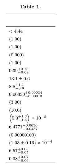
which, when dropped into a proper LaTeX document, results in the following table:
This is not a particularly fancy-looking table, but it gets the essential bits: numbers, in the right places, with error bars, and some sort of indication when a parameter is frozen.
A slightly less simple example: A table with row and column names
With a little extra work, we can make this look better:
isis> load_par("best.err");
isis> variable parndx = [1,[6:9],[12:17]]; % select which parameters we want in the table
isis> variable p = get_params(parndx);
isis> variable rownames = array_struct_field(p,"name"); % get the names of the parameters for the row names
isis> rownames = array_map(String_Type,&strreplace,rownames,"_","\\_"); % Change _ to \_ so LaTeX doesn't complain
isis> variable colnames = ["Parameter","Value"];
isis> variable lab = "tab:example"; % the label that the table with receive
isis> variable caption = "Example table!"; % the caption for the table
isis> variable t = sltable(p;rownames=rownames,label=lab,caption=caption);
isis> variable f = fopen("example.tex","w+");
isis> () = fputs(t,f);
isis> () = fclose(f);
This results in the following LaTeX file:
\begin{deluxetable}{lr}
  \tabletypesize{\footnotesize}
  \tablewidth{0pt}
  \tablecaption{The best-fit parameters\label{tab:best}}
  \tablehead{\colhead{Parameter}&\colhead{Value}}
  \startdata
    tbnew\_feo(1).nH & $< 4.44$ \\
    powerlaw(1).PhoIndex & $0.39^{+0.16}_{-0.09}$ \\
    highecut(1).cutoffE & $13.1\pm0.6$ \\
    highecut(1).foldE & $8.8^{+1.1}_{-0.8}$ \\
    enflux(1).enflux & $0.00330^{+0.00034}_{-0.00013}$ \\
    gaussian(1).norm & $\left(5.3^{+1.3}_{-1.4}\right)\times10^{-5}$ \\
    gaussian(1).LineE & $6.4771^{+0.0030}_{-0.0487}$ \\
    gaussian(1).Sigma & $(0.00000100)$ \\
    gaussian(2).norm & $\left(1.03\pm0.16\right)\times10^{-4}$ \\
    gaussian(2).LineE & $6.57^{+0.06}_{-0.05}$ \\
    gaussian(2).Sigma & $0.38^{+0.07}_{-0.06}$ \\
  \enddata
\end{deluxetable}
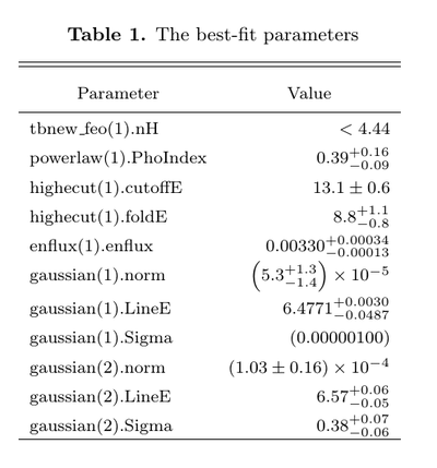
which looks like this once compiled:
Much nicer!
A significantly less simple example: Multiple datasets, same model
Often we want to include tables with multiple sets of parameters - for example, you have multiple observations fit with the same model, and you want to show them all in the same table. I have four files, 10145-01-01-00.par, 20146-07-02-00.par, 50067-03-01-00.par, and 80016-02-01-00.par, which have the best-fit parameters with uncertainties for four RXTE observations of the HMXB 4U 1538-522. They all look something like this:
constant(Isis_Active_Dataset)*tbnew_feo(1)*(enflux(1,powerlaw(1)*highecut(1)*gauabs(1)*gauabs(2))+egauss(1)+egauss(2))
# [bgd 1] = fcorback(1)
# [bgd 2] = fcorback(2)
 idx  param              tie-to  freeze         value         min         max
  1  constant(1).factor      0     1                1           1           1
  2  tbnew_feo(1).nH         0     0         3.973725    3.658599    4.266751  10^22
  3  tbnew_feo(1).O          0     1                1           1           1
  4  tbnew_feo(1).Fe         0     1                1           1           1
  5  tbnew_feo(1).redshift   0     1                0          -1          10
  6  powerlaw(1).norm        0     1                1           1           1
  7  powerlaw(1).PhoIndex    0     0         1.285706    1.270116    1.300309
  8  highecut(1).cutoffE     0     0         14.56784    13.48842    15.39921  keV
  9  highecut(1).foldE       0     0         11.22298    9.676076    13.51359  keV
 10  gauabs(1).E0            0     0         20.52605    19.97606    21.16913  keV
 11  gauabs(1).Sigma         0     0          2.32501    1.487142    2.731347  keV
 12  gauabs(1).Depth0        0     0        0.4493259   0.3621914   0.5180218
 13  gauabs(2).E0            0     1                6           6           6  keV
 14  gauabs(2).Sigma         0     1             0.01        0.01        0.01  keV
 15  gauabs(2).Depth0        0     1                0           0         0
 16  enflux(1).enflux        0     0        0.5329864   0.5183991   0.5502475  keV/s/cm^2
 17  enflux(1).E_min         0     1                3           3           3  keV
 18  enflux(1).E_max         0     1               50          50          50  keV
 19  egauss(1).area          0     0     0.0001673404  0.0001109895  0.0002221102  photons/s/cm^2
 20  egauss(1).center        0     1              6.4         6.4         6.4  keV
 21  egauss(1).sigma         0     1             0.01        0.01        0.01  keV
 22  egauss(2).area          0     0    -0.0001235576  -0.0002494129           0  photons/s/cm^2
 23  egauss(2).center        8     0         14.56784          10          25  keV
 24  egauss(2).sigma         0     1             0.01        0.01        0.01  keV
 25  constant(2).factor      0     0         1.001348   0.9384046    1.052464
 26  fcorback(1).norm        0     0        0.9637407    0.954889   0.9701586
 27  fcorback(1).id          0     1                1           1           1
 28  fcorback(2).norm        0     0         1.000418   0.9945778    1.006313
 29  fcorback(2).id          0     1                2           2           2
To make a table with all four, I have the following script:
variable obs = ["10145-01-01-00","20146-07-02-00","50067-03-01-00","80016-02-01-00"];
variable i;
% We need to load some data so the model parameters can be loaded. Literally
% any set of two spectra will work just fine - this is just so the
% constant(Isis_Active_Dataset) component can be loaded properly.
clear_all(;noprompt);
load_data("/opt/data/rxte/H1538/phase_averaged/103-123/10145_pca_103-123.pha");
load_data("/opt/data/rxte/H1538/phase_averaged/103-123/10145_hexte_103-123.pha");
% The arrays of structs will be stored in a list:
variable p = list_new();
% These are the indices of the parameters I want to include in the table, in
% the order I want them to appear:
variable parndx = [16,25,2,[7:12],19,22];
% Here are fancy names for the parameters listed in parndx:
variable parname = ["Flux","$C_{\\rm HEXTE}$","$N_{\\rm H}$",
  "$\\Gamma$","$E_{\\rm cut}$","$E_{\\rm fold}$",
  "$E_{\\rm cyc}$","$\\sigma_{\\rm cyc}$","$\\tau_{\\rm cyc}$",
  "$A_{\\rm Fe}$","$A_{\\rm smooth}$"];
% And their units:
variable parunits = ["keV\\,cm$^{-2}$\\,s$^{-1}$","","$\\times 10^{22}$\,cm$^{-2}$",
  "","keV","keV","keV","keV","","$\\times 10^{-4}$\\,ph\\,cm$^{-2}$\\,s$^{-1}$",
  "$\\times -10^{-4}$\\,ph\\,cm$^{-2}$\\,s$^{-1}$"];
% Loop through the observations, loading the parameters, doing some processing
% and rescaling to make things look better on the page, and storing them in the
% list:
_for i (0,length(obs)-1,1) {
  load_par(obs[i]+".par");
  variable ptemp = get_params(parndx);
  % The iron line and "smoothing" Gaussian (egauss(1) and egauss(2)) get scaled
  % up by 1e4 (note that I've noted that in their units above)
  ptemp[-2].value *= 1e4;
  ptemp[-2].min *= 1e4;
  ptemp[-2].max *= 1e4;
  % The "smoothing" Gaussian additionally has a negative normalization - we
  % flip the sign here (this means we need to swap the min and max fields, too)
  ptemp[-1].value *= -1e4;
  ptemp[-1].min *= -1e4;
  ptemp[-1].max *= -1e4;
  variable temp = @ptemp[-1].max;
  ptemp[-1].max = @ptemp[-1].min;
  ptemp[-1].min = temp;
  % "ptemp" is an array of structs, which we append to the list "p"
  list_append(p,ptemp);
}

% Note the use of __push_list() to push the list "p" onto the stack. This is
% the equivalent of writing "sltable(p[0],p[1],p[2],p[3])", but with the
% advantage that it works no matter how many elements "p" has.
variable t = sltable(__push_list(p);
  rownames = {parname,parunits},  % a List_Type here is interpreted as parameter names and units
  colnames = obs, % names for columns
  notes = {["Energy frozen to 6.4\\,keV, width frozen to 0.01\\,keV"],["*"]}, % note use of List_Type here too
  caption = "Fits to 4U~1538$-$522 for four \\textit{RXTE} ObsIDs", % caption
  label = "tab:multiple"); % label

% Write the table to a file
variable f = fopen("multiple.tex","w+");
() = fputs(t,f);
() = fclose(f);
This is quite a bit of code, but the actual code to make the table itself is, again, only one line. The resulting multiple.tex file looks like this:
\begin{deluxetable}{lrrrrr}
  \tabletypesize{\footnotesize}
  \tablewidth{0pt}
  \tablecaption{Fits to 4U~1538$-$522 for four \textit{RXTE} ObsIDs\label{tab:multiple}}
  \tablehead{& & \colhead{10145-01-01-00}&\colhead{20146-07-02-00}&\colhead{50067-03-01-00}&\colhead{80016-02-01-00}}
  \startdata
    Flux & keV\,cm$^{-2}$\,s$^{-1}$ & $0.533^{+0.018}_{-0.015}$ & $0.700^{+0.016}_{-0.006}$ & $0.805^{+0.013}_{-0.005}$ & $0.493^{+0.021}_{-0.019}$ \\
    $C_{\rm HEXTE}$ &  & $1.00^{+0.06}_{-0.07}$ & $0.81\pm0.04$ & $0.811\pm0.023$ & $0.79\pm0.06$ \\
    $N_{\rm H}$ & $\times 10^{22}$,cm$^{-2}$ & $3.97^{+0.30}_{-0.32}$ & $1.55^{+0.21}_{-0.14}$ & $1.87^{+0.19}_{-0.18}$ & $2.4\pm0.6$ \\
    $\Gamma$ &  & $1.286^{+0.015}_{-0.016}$ & $1.170\pm0.013$ & $1.160^{+0.011}_{-0.012}$ & $1.078^{+0.026}_{-0.027}$ \\
    $E_{\rm cut}$ & keV & $14.6^{+0.9}_{-1.1}$ & $14.8\pm0.5$ & $14.9\pm0.4$ & $14.0^{+0.6}_{-0.5}$ \\
    $E_{\rm fold}$ & keV & $11.2^{+2.3}_{-1.6}$ & $11.3^{+1.1}_{-0.6}$ & $11.1^{+0.7}_{-0.5}$ & $10.5^{+1.6}_{-1.4}$ \\
    $E_{\rm cyc}$ & keV & $20.5^{+0.7}_{-0.6}$ & $20.72^{+0.32}_{-0.05}$ & $20.84^{+0.23}_{-0.22}$ & $20.9\pm0.7$ \\
    $\sigma_{\rm cyc}$ & keV & $2.3^{+0.5}_{-0.9}$ & $2.81^{+0.21}_{-0.16}$ & $2.92\pm0.22$ & $2.6^{+0.6}_{-0.7}$ \\
    $\tau_{\rm cyc}$ &  & $0.45^{+0.07}_{-0.09}$ & $0.51\pm0.06$ & $0.52^{+0.04}_{-0.05}$ & $0.54\pm0.12$ \\
    $A_{\rm Fe}$ & $\times 10^{-4}$\,ph\,cm$^{-2}$\,s$^{-1}$ & $1.7\pm0.6$ & $4.2^{+0.6}_{-0.5}$ & $5.2\pm0.6$ & $4.3\pm1.0$ \\
    $A_{\rm smooth}$ & $\times -10^{-4}$\,ph\,cm$^{-2}$\,s$^{-1}$ & $< 2.49$ & $1.7^{+0.9}_{-0.6}$ & $2.2^{+0.7}_{-0.8}$ & $< 0.748$ \\
  \enddata
  \tablenotetext{*}{Energy frozen to 6.4\,keV, width frozen to 0.01\,keV}
\end{deluxetable}
Two things to note here: sltable() will produce one column of numbers for each array of structs you give it, so the use of a list variable and push_list lets us make tables with arbitrary numbers of columns fairly easily. Second, the "notes" qualifier takes a two-element List_Type: the first element is an array of string containing the text of the notes, and the second element is an array of strings containing the symbols for those notes.
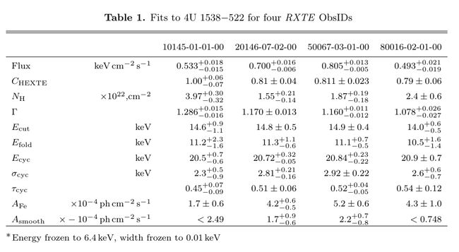
The table, once compiled with LaTeX, looks like this:
For a good time, try adding the qualifiers "horiz=1,landscape=1" and swapping the "rownames" and "colnames" qualifiers. You should get something like this:
There is one issue, which is that the footnote should be accompanied by a marker on the iron line area (i.e., A_Fe should have an asterisk next to it). I haven't figured out a sensible way to approach this, so right now you'll have to add those in by hand.
A decidedly not simple example: Multiple different models
If you are making a table with multiple models (that is, models with different sets of parameters), you need to inform sltable() that it needs to plot rows where some columns have no data. This is where the "nodata" field for the input structure comes into play.
Say you have an array of parameter names (or some sort of identifier; let's call that variable parnames) that you want to include in a table, and you have arrays of structures returned by get_params() from a few different models (let's call those m1 and m2 here). The way I've approached this is to create a new list of arrays of structures, tableParams, that will be the input to sltable(), with extra rows with the "nodata" field set to 1 for missing parameters. We loop over all the parameters, and if the parameter is included in the model, we copy that structure into tableParams; if the parameter is not present, we set that element of tableParams to a structure with nodata = 1.
variable i,j;
variable models = {m1,m2};
variable modelNames = ["model 1","model 2"];
variable nModels = length(models);
variable tableParams = List_Type[nModels];
_for j (0,nModels-1,1) {
  _for i (0,length(parnames)-1,1) {
    if(length(where(array_struct_field(models[j],"name") == parnames[i])) == 1) {
      tableParams[j][i] = struct_copy(models[j][i]);
    } else {
      tableParams[j][i] = struct{value=0.0,nodata=1};
    }
}
variable t = sltable(__push_list(tableParams);rownames=array_struct_field(tableParams[0],"name"),colnames=modelNames);
You could do this with a 1D or 2D array of structures, but I find the "list of arrays" approach is easier to keep track of (and it's not like efficiency is incredibly important for this task anyway...).
By default this outputs a \nodata command for deluxetable tables and an \ldots command for a tabular table, but you can customize this by setting the nodata qualifier for sltable() to your preferred string.


