Isis tutorial walkthrough
A Walk Through ISIS
In this first part of the tutorial, in order to get you started we will show you an example for a full X-ray data analysis using a fairly simple spectrum[1].
In the following tutorial, we will be working on a simple data set from an observation of a black hole, Cygnus X-1, that was obtained with NASA's Rossi X-ray Timing Explorer satellite. The test data set can be downloaded from here. It consists of the following parts:
standard2f_0134off_top.pha-- the spectrum itself.standard2f_back_SkyVLE_top_good_0134off.pha-- The background spectrum (referred to in theBACKFILEkeyword ofstandard2f_0134off_top.pha; see later for explanations).p2_LR1_2009-05-06.rsp-- The response matrix (referred to in theRESPFILEkeyword ofstandard2f_0134off_top.pha; see later for explanations)
The data are in FITS-format, a standard file format that is used in all of astronomy. Right now you can treat these files as a black box, at the end of this document there is some additional information about how to inspect the contents of these files outside of isis.
Invoking isis
Isis is a command-line program and is therefore usually executed from the command line (the details are explained in the installation instructions):
wilms@leo:~> isis
which then prints out some start up messages before you end with the isis prompt:
Welcome to ISIS Version 1.6.2-44
Copyright (C) 1998-2020 Massachusetts Institute of Technology

          Isis web page: http://space.mit.edu/cxc/isis/
   Mailing list archive: http://space.mit.edu/cxc/isis/archive/
 Send questions to the mailing list: <isis-users@space.mit.edu>.
     For a summary of recent changes, type:  "help changes"

isis>
As part of its startup, isis executes a file called .isisrc, which is useful for setting up a standard environment.
In the following we will show you an interactive session with isis. It is the typical approach when working with new data to look at these first by hand, in a way similar to that shown here. In later, more advanced analysis you will probably mainly interact with isis through programs, although it should be emphasized that working interactively with data first is always a good idea. This is the only way how you can get a good feeling for your data, even though automated reductions are important, especially when working on data sets with many different observations.
For a more formal walk through through isis and the programming language s-lang, take a look at the isis web page, especially the documentation available there.
Loading and Inspecting Your Data Set
We now load the data we looked at before into isis:
pca=load_data("standard2f_0134off_top.pha");
The load_data command loads the file given as its argument and returns an unique number that identifies this data set. In the above example, this identifier is stored in the variable called pca (it usually makes sense to use the name of the detector with which the data were taken, although there are exceptions). Note that the command ends with a semicolon. This is standard in slang, the language on which isis is based. Although it is in principle possible to switch off this feature when working interactively with isis[2], we recommend you do not use this option -- having to type the semicolon requires you to think before doing something, which is generally a good idea ;-).
If all goes fine, you will be informed that the response matrix includes the ARF. Now check whether isis loaded what you think it should have loaded by looking at some basic information about the background file, the RMF, and the ARF:
isis> list_data;
Current Spectrum List:
 id    instrument part/m  src    use/nbins   A   R     totcts   exp(ksec)  target
  1           PCA          0     129/  129   -   1  3.1773e+06     2.528  CYG_X-1
file:  standard2f_0134off_top.pha
back:  standard2f_back_SkyVLE_top_good_0134off.pha
Amongs others, the table columns include
id: the identifier of this data set,nbins: the number of spectral bins,totcts: the total counts in the spectrum,exp: the exposure time in kiloseconds, andtarget: the nominal source we are working with.
Finally, the output also lists the file name and the associated background file.
Similar information can also be obtained for the response matrix and the ARF using the commands
list_rmf;
list_arf;
Note that for your data set no information is given back for the ARF, since none was loaded.
Like for all commands in isis, information about the commands can be obtained with
isis> help commandname
so, for example,
isis> help list_arf
(If this does not give you help for the command you put in, you can try just
isis> commandname;
without any additional arguments. For some commands that works.)
Some of the help information might appear pure gibberish for you. Ignore this for the moment, with time it will all become clear to you.
A second help function that is very useful is the apropos command. For example, if you want to do something with an ARF, do
isis> apropos arf
which will return all isis commands that contain "arf" in their name.
Exercise 1
- Load your data set and check the information given by ISIS using the above commands.
Plotting the Data
X-ray data analysis of a data set that you do not yet know consists basically of the following steps:
- plot something
- think about what the plot/data set tries to tell you
- try something out (e.g., perform a fit)
- goto 1
and then repeat until you are convinced that everything works as expected. Depending on the data set, the above might take five minutes, but we also had complicated data sets that so far have resulted in 2-3 PhD theses...
Therefore, as the first step, we take a look at our data.
While isis contains some basic plotting routines, it is generally faster to use the very powerful plotting routines developed at MIT and at Remeis/ECAP to look at the data. The reason is that these are more user friendly than the basic isis routines.
In order to do so, we first need to load the Remeis isis scripts. In our standard install, just do a
isis> require("isisscripts");
The isisscripts are a large set of useful routines developed by many people. If you use them for professional work, please contact J. Wilms first and ask whom to put in the acknowledgments of your paper. They are freely available through a git-repository.
So let's plot the data set:
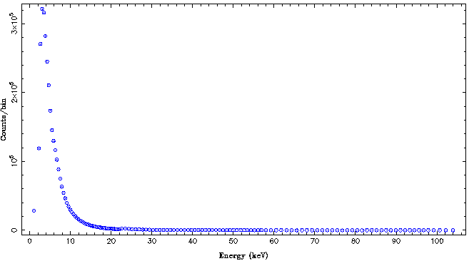
isis> plot_counts(pca);
A window pops up, looking something like this
In this standard display, not much can be seen except for the fact that the detector sensitivity is the best at low energies. For this reason, we first switch the plot over to a log-log plot and plot again:
isis> xlog;
isis> ylog;
isis> plot_counts(pca);
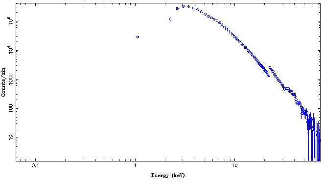
This results in a much nicer plot. With the exception of gratings data, it is usually better to take a look at X-ray data in log-log space, so you should get used to switching over to log-space before doing any plots:
Note that what is shown are counts per PHA bin as a function of energy. Here, the response matrix is used to get an approximate conversion of the channel number to energy. The jump at around 20keV is not a spectral feature, but caused by the detector: at this energy, the standard data mode on RXTE PCA increases the energy width per PHA bin by a factor of two. Since the spectrum changes only slowly at this energy, because of the increase in width twice as many counts are detected in this bin. In addition, the feature at around 30keV is also a detector feature, it mainly reflects the change in sensitivity of this Xe-based proportional counter at the Xe-K-edge, which is at roughly 30keV.
Experience for this detector shows that its calibration is best at energies between 3keV and 22keV, such that for the moment we will ignore what is happening outside of this energy band using isis' notice function:
isis> notice_values(pca,3.,22.;unit="keV");
isis> plot_counts(pca);
Note that immediately after ignoring, we plot the data again in order to make sure that our command worked as intended. This way you can visually confirm, e.g., that a feature that you want to ignore really was outside of the energy range considered. Furthermore, note that we are explicitly telling isis to work in energy space. This is necessary since for historic reasons many isis commands are by default working in wavelength space.
Other useful isis commands for noticing and ignoring energy and wavelength ranges are
ignore(id);         % Ignore dataset id
notice(id,a,b);     % Notice wavelength range [a,b] in dataset id
notice_en(id,a,b);  % Notice energy range [a,b] in dataset id
xnotice(id,a,b);    % *Only* notice wavelength range [a,b] in dataset id
xnotice_en(id,a,b); % *Only* notice energy range [a,b] in dataset id
exclude(id);        % Don't change the ignored/noticed channels, but
                    % exclude the whole data set until reinstated with:
include(id);        % Reinstate the data with prior excluded channels
You can get more information about all of these commands with the .help-command. Note that all of the above commands are "inclusive", in the sense that the energy bins in the spectrum that include the two borders, a and b, are contained in the noticed energy band.
Exercise 2
- Perform the above steps for your data set. In the write up of your homework, include the relevant figures. Prepare these figures as publication-quality (postscript) figures. For this you will have to switch the output to postscript before plotting, and switch back to screen output afterwards:
isis>plotid = open_print("example.ps/vcps");
isis> keynote_size; nice_width;
isis> plot_counts(pca);
isis> close_print(plotid);
where example.ps is the file name of the postscript file, and where keynote_size and nice_width set the size of the figure to something that is appropriate for inclusion into a journal article. If you rather work with pdf, convert the ps-file to pdf afterwards, e.g., using Linux epstopdf program.
Inspecting ARF and RMF
It is always useful in data analysis to have a feeling for the major features introduced by specific properties of the detector used to measure the data. For example, in the spectra above there are drops in detector sensitivity at the K- and L-edges of the detector gas. Usually, the regions around these edges are less well calibrated. Visualizing the ARF and RMF helps in this case (as does reading the user's manual for the satellite you're using...).
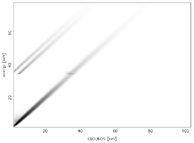
It is easy to produce a plot of the RMF:
isis> fits_plot_rmf("p2_LR1_2009-05-06.rsp");
The resulting plot should be similar to this:
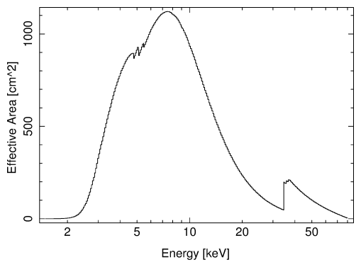
To visualize the sensitivity of the detector we need to plot the effective area of the detector as a function of energy. Depending on the instrument, the detector sensitivity is either saved as a separate ARF (Ancilliary Response File) or it is stored as part of the RMF. In the latter case isis will tell you so with the warning message "RMF includes the effective area" when you load the response. In this case we need to factor the response first:
isis> rsp=load_rmf("p2_LR1_2009-05-06.rsp");
RMF includes the effective area
isis> arf=factor_rsp(rsp);
We can then get the information about the effective area and plot it:
isis> arfdata=get_arf(arf);
isis> xlog;
isis> hplot(_A(arfdata));
where the function _A converts the wavelength information contained in the structure arfdata to keV.
Performing a First Spectral Fit
We are now ready to perform a first spectral fit. We first need to define the spectral model that we want to describe our data with. In general, one first tries to get a rough description of the data, which is for example based on earlier observations of the object and general astrophysical knowledge about the class of objects - if present -, and then refines this spectral model by adding further spectral components if an initial fit was successful. Isis includes a large number of spectral models. Since the models are derived from XSPEC, a good overview is given by the exhaustive list of the models in the XSPEC manual.
What model to use depends on the object one looks at. In most cases, one tries either a power law or a black body first and only later works with more CPU-intensive, physics-based models. Since all X-ray sources are absorbed by the interstellar medium in our Galaxy, one always includes Galactic absorption.
Here, we know that Cygnus X-1 is a black hole. These often have power-law spectra. We therefore start by trying an absorbed power-law as our fit function:
isis>fit_fun("tbabs(1)*powerlaw(1)");
Notice the numbers behind the model components. These will be later used to distinguish different fit-functions, e.g., when one works with a source that has a spectrum that can be described as the sum of two power laws of different photon indices.
Next we take a look at our fit parameters:
isis> list_par;
tbabs(1)*powerlaw(1)
 idx  param             tie-to  freeze         value         min         max
  1  tbabs(1).nH            0     0                1           0      100000  10^22
  2  powerlaw(1).norm       0     0                1           0       1e+10
  3  powerlaw(1).PhoIndex   0     0                1          -2           9
Amongst other information, which we will be discussing in a later tutorial, the table contains the following information:
idx: The index of the parameter (see below)param: The name of the parameter. For example,tbabs(1).nHis the absorption column (in units of 10^22 cm-2. The physical meaning of the parameters is explained in the XSPEC manual.tie-toandfreeze: see latervalue: the current value of the parameterminandmax: The fit has to remain in the range between these two values.
Before we do our first fit, we take a look at how this model looks like when folded through the detector response matrix. In order to do so we first ask isis to change the model flux such that the predicted count rate is close to the model count rate.
isis> renorm_counts;
:
 Parameters[Variable] = 3[1]
            Data bins = 45
           Chi-square = 898942.6
   Reduced chi-square = 20430.51
0
Isis has changed the parameter powerlaw(1).norm and has left all other parameters unchanged:
isis> list_par;
tbabs(1)*powerlaw(1)
 idx  param             tie-to  freeze         value         min         max
  1  tbabs(1).nH            0     0                1           0      100000  10^22
  2  powerlaw(1).norm       0     0        0.4145608           0       1e+10
  3  powerlaw(1).PhoIndex   0     0                1          -2           9
Now let us take a look at what the model looks like
isis> plot_counts(pca);
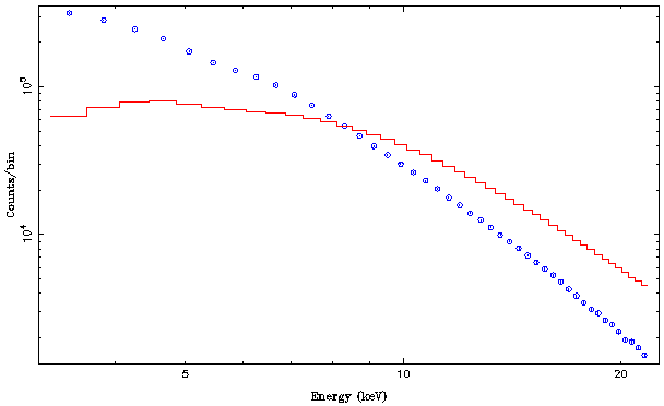
The resulting plot looks something like this:
Notice that the slope of the spectrum and the data is very different. With a photon index of 1 the spectrum is harder than the data. We therefore change the photon index to something that is more typical for black holes, renorm the spectrum and plot it again:
isis> set_par(3,1.7);
isis> renorm_counts;
 Parameters[Variable] = 3[1]
            Data bins = 45
           Chi-square = 339671.5
   Reduced chi-square = 7719.808
0
isis> plot_counts(pca);
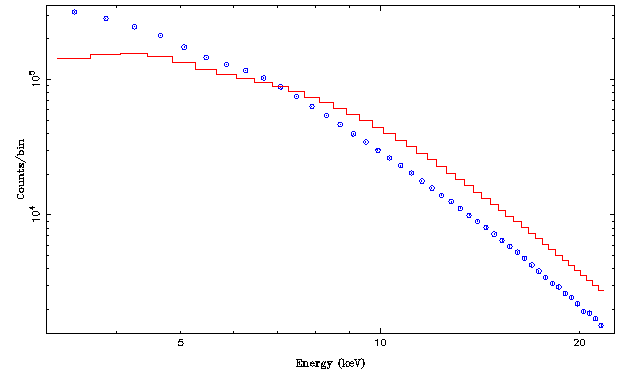
The resulting model looks like this:
Note that the overall slope now looks ok, but there is still some deviation between the data and the model at the soft part of the spectrum, where the model looks too much absorbed. Taking a look at the isis help for set_par, we are being told that instead of changing the parameter by giving set_par its index number, we could also have given the full name of the parameter. So let us remove some absorption to get the curvature at the low energies right, by setting NH to its interstellar value of <latex>N_\mathrm{H}=3\times 10^{21}\,\mathrm{cm}^{-2}</latex>.
isis> set_par("tbabs(1).nH",0.3);
isis> renorm_counts;
 Parameters[Variable] = 3[1]
            Data bins = 45
           Chi-square = 314595.1
   Reduced chi-square = 7149.888
0
isis> plot_counts(pca);
Note that the Chi-square value decreased, meaning that the new description of the model is slightly better than the previous one.
We now have starting values that are good enough to start the proper fitting. Here isis is using a so-called Levenberg-Marquardt-gradient method to minimize chi-square by varying the parameters. This is done step by step, until a (possibly local) minimum is reached. In order to see how the parameters are being varied, we instruct isis to display all intermediate parameter values first, and then perform the fit:
isis> Fit_Verbose=1;
isis> fit_counts();
chisqr= 3.1460e+05:
 tbabs(1).nH=  3.00000000e-01 powerlaw(1).norm=  2.26407499e+00
 powerlaw(1).PhoIndex=  1.70000000e+00
chisqr= 3.1460e+05:
 tbabs(1).nH=  3.00030000e-01 powerlaw(1).norm=  2.26407499e+00
 powerlaw(1).PhoIndex=  1.70000000e+00
:
: multiple further steps
:
chisqr= 9.6239e+03:
 tbabs(1).nH=  0.00000000e+00 powerlaw(1).norm=  1.32707632e+01
 powerlaw(1).PhoIndex=  2.61135748e+00
chi-square value converged
 Parameters[Variable] = 3[3]
            Data bins = 45
           Chi-square = 9623.869
   Reduced chi-square = 229.1397
0
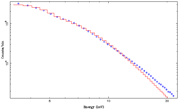
While the reduced chi-square is already much smaller, it is still very much above its ideal value of around unity. Let us take a look what the current best fit looks like by plotting it again:
The model describes the overall shape of the data rather well, but statistically significant residuals remain. We will tackle these in the next section, but first let us save our work so far such that we can start again from the current best fit in case our next steps are not successful:
isis> save_par("powerlaw.par");
This creates a file called powerlaw.par that can be re-read later using
isis> load_par("powerlaw.par");
The file is a simple ASCII file that you can either just display on screen (using the unix-command cat powerlaw.par from the shell or any editor of your choice.
Exercise 3
- Perform the procedure described above with "your" data set, documenting all steps.
- If you want to change more than one parameter at a time, instead of using
set_paryou can also use theedit_parfunction, which will invoke an editor of your choice with a table like the parameter table above. You can then overwrite all values with your new values, save this temporary file, and exit the editor. Try this with your data set.
Improving the Initial Fit
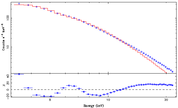
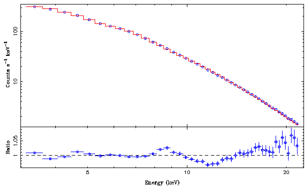
Now that we have an initial fit, we can take a closer look at the difference between the data and the model to get a feeling what we can do to improve the model. Since the data values and the model are already rather close together, guessing what is going on by looking at the slight differences between both is not very useful. We therefore plot our data again, but this time not only displaying the data but also the "residuals", that is the difference between the data and the model:
isis> plot_data(pca;res=1);
This results in the following figure:
Note the following:
- instead of using
plot_countswe have usedplot_data(which is in reality an alias for theplot_data_countsfunction).plot_datadisplays the counts and the model in terms of counts per keV, while previously we used counts per PHA bin. This is the preferred way to plot X-ray data, since it is slightly closer to showing the proper spectrum thanplot_counts. - Secondly, in addition to plotting the data we are also plotting the residuals, by using the "qualifier"
res=1. In Slang/isis, qualifiers are special switches in functions. They all have names (resin the above example), i.e., the order in which they are listed after the initial semicolon does not matter. The most important ways of displaying residuals areres=1: Display the residual in terms of chi, i.e., display the value of <latex>(data-model)/\sigma</latex> where <latex>\sigma</latex> is the statistical uncertainty of the bin.res=3: Display the ratio between the data and the model, <latex>data/model</latex>.
- other qualifiers that are useful in plotting are:
mcol=number: the color of the model, number is, well, a number. Avoidmcol=3andmcol=5since these colors do not show up on beamers.dcol=number: dito, for the datadecol=number: dito, for the error barsbkg: ifbkg=0then plot the data with the background subtracted, ifbkg=1also show the background (this will be useful later).xrange={min,max}: plot the x-axis from min to max only. Note the curly braces! Setminand/ormaxtoNULLif you want to reset this range to its default value. It is important to remember thatxrangejust sets the plot-range, you need to usenoticeto set the energy range that is used for fitting.yrange={min,max}: dito, for the y-axis.
As an example, try
isis> plot_data(pca;res=1,mcol=2,dcol=1,decol=5);
The residuals in the plot tell us two things:
 - there is a "bump" around 6.4keV. This is typically an indication that there is an iron Kα line present around 6.4keV.
 - there is a "soft excess" at low energies, which might be indicative of an accretion disk.
Looking at the XSPEC manual tells us that accretion disk spectra are modeled with the diskbb model while emission lines are modeled using the gauss model. However, reading the isis manual tells us that the only model that has a different name in isis and in XSPEC is gauss where we will have to use egauss instead.
Based with this information we setup the new fit function as follows
isis> fit_fun("tbabs(1)*(diskbb(1)+egauss(1)+powerlaw(1))");
and identify the new parameters with list_par:
isis> list_par;
tbabs(1)*(diskbb(1)+egauss(1)+powerlaw(1))
 idx  param             tie-to  freeze         value         min         max
  1  tbabs(1).nH            0     0                0           0      100000  10^22
  2  diskbb(1).norm         0     0                1           0       1e+10
  3  diskbb(1).Tin          0     0                1           0        1000  keV
  4  egauss(1).area         0     0                1           0           0  photons/s/cm^2
  5  egauss(1).center       0     0                1           0           0  keV
  6  egauss(1).sigma        0     0            0.002       1e-06           1  keV
  7  powerlaw(1).norm       0     0         13.27076           0       1e+10
  8  powerlaw(1).PhoIndex   0     0         2.611357          -2           9
We then set the center of the Gaussian to 6.4keV (set_par(5,6.4);) and plot again. Nothing changes. The reason is that we first have to tell isis to recalculate the model. Not doing this automatically after every invocation of set_par makes sense since some models might take up large amounts of CPU time. To recalculate the model, use
isis> eval_counts;
Plot the model again (using plot_data). You will notice that the Fe line is too strong. Reduce its flux accordingly by changing the area parameter. You will probably need a few attempts to get something that looks ok. Then repeat this procedure with the parameters of the accretion disk until you get something that looks halfway ok. Save this attempt, just to be on the save side, and then perform a fit.
Repeating the above a few times, I managed to coax the following best fit out of the data
isis> list_par;
tbabs(1)*(diskbb(1)+egauss(1)+powerlaw(1))
 idx  param             tie-to  freeze         value         min         max
  1  tbabs(1).nH            0     0                0           0      100000  10^22
  2  diskbb(1).norm         0     0          4088.32           0       1e+10
  3  diskbb(1).Tin          0     0        0.7163385           0        1000  keV
  4  egauss(1).area         0     0       0.07462147           0           0  photons/s/cm^2
  5  egauss(1).center       0     0         6.085836           0           0  keV
  6  egauss(1).sigma        0     0                1       1e-06           1  keV
  7  powerlaw(1).norm       0     0         2.948465           0       1e+10
  8  powerlaw(1).PhoIndex   0     0         1.984697          -2           9
with
Parameters[Variable] = 8[8]
            Data bins = 45
           Chi-square = 291.7067
   Reduced chi-square = 7.883964
This fit looks the following:
This is quite ok for such a simple model. Note that there still is some hardening above 10keV and the residuals are not perfect around 8keV either. This is due to the too large width of the simple Gaussian line, limitations in the diskbb-model, and the fact that in this data set the source was in its intermediate state, where the combination of the disk component and the power law is notoriously hard to model.
Exercise 4
- you guessed it: try to find a good fit for your data set.
Inspecting your data set outside of isis
You can take a look at what such a file looks like using the fv or fdump programs, which are part of HEASOFT and should already be installed on your machine. Outside of isis, invoke fv with
fv standard2f_0134off_top.pha
A window pops up that displays the contents of the file. Like all FITS files PHA[3] files consist of a so-called primary-header and then multiple extensions, which again contain some human-readable header data that contain information about your data set and the data itself. The header information is given as a keyword name, the value of the keyword, and often a comment that describes the meaning of the keyword. Important keywords are
OBJECT: The name of the observed object (a string defined by the observer, often - but not always - a meaningful name)RA_OBJandDEC_OBJ: The position of the object (often useful if theOBJECT-keyword is not set or wrong)TELESCOPandINSTRUME: The satellite and instrument usedDATE-OBSandDATE-END: The date and time of the start and the end of the observationEXPOSURE: The exposure time, i.e., how long were data accumulated. Note that oftenEXPOSUREis smaller than the difference betweenDATE-OBSandDATE-ENDsince the detector could have been switched off for part of the observation, or data were discarded during the data reduction, e.g., because of large background fluxes[4].BACKFILE: The name of the PHA-file that defines the background, which is automatically subtracted from the data before fitting.RESPFILE: The name of the file containing the detector response matrix (often called "RMF" or "RSP", which describes the mapping from PHA-space to energy space and all detector effects.ANCRFILE: The name of the ancilliary response file, often called ARF-file. This file is used by some instruments which separate the detector response into a pure energy redistribution matrix and an effective area. See the X-ray astronomy lectures for details. This keyword has the valueNONEif the ARF is already part of the response matrix.- Further keywords depending on the satellite (often one finds, e.g.,
TSTARTandTSTOPwhich contain the same information asDATE-OBSandDATE-END, only in a system that is easier to use in calculation than the human-readable information inDATE-OBSandDATE-END).
standard2f_back_SkyVLE_top_good_0134off.pha: The background spectrum referred to in theBACKFILEkeyword ofstandard2f_0134off_top.phap2_LR1_2010-07-04.rsp: The response matrix referred to in theRESPFILEkeyword ofstandard2f_0134off_top.pha
As mentioned above, you can either take a look at the files with fv, or by dumping the FITS-file on the screen using the fdump command. Here is the output of the latter, showing typical values of the keywords above:
wilms@leo:~/isistut> fdump standard2f_0134off_top.pha
Name of optional output file[STDOUT]
Names of columns[]
Lists of rows[-]
SIMPLE  =                    T / file does conform to FITS standard
BITPIX  =                  -32 / number of bits per data pixel
NAXIS   =                    0 / number of data axes
EXTEND  =                    T / FITS dataset may contain extensions
COMMENT   FITS (Flexible Image Transport System) format is defined in 'Astronomy
COMMENT   and Astrophysics', volume 376, page 359; bibcode: 2001A&A...376..359H
:
: ... many further lines
:
XTENSION= 'BINTABLE'           / binary table extension
BITPIX  =                    8 / 8-bit bytes
:
:
EXTNAME = 'SPECTRUM'           / name of this binary table extension
:
TELESCOP= 'XTE     '           / Telescope (mission) name
INSTRUME= 'PCA     '           / Instrument name
FILTER  = 'NONE    '           / Instrument filter in use
EXPOSURE= 2.52800000000001E+03 / Exposure time
:
BACKFILE= 'standard2f_back_SkyVLE_top_good_0134off.pha' / Background FITS file f
CORRFILE= 'standard2f_back_SkyVLE_top_good_0134off.pha' / Correlation FITS file
RESPFILE= 'p2_LR1_2010-07-04.rsp' / Redistribution matrix file (RMF)
ANCRFILE= 'NONE    '           / Ancillary response file (ARF)
:
CREATOR = 'SAEXTRCT version 4.2g' / Program name that produced this file
DATE    = '2011-06-26T10:08:03' / file creation date (YYYY-MM-DDThh:mm:ss UT)
RA_OBJ  =       2.99591705E+02 / RA of First input object
DEC_OBJ =       3.52016983E+01 / DEC of First input object
EQUINOX =              2000.00 / Equinox of the FIRST object
:
DATASUM = '3317156129'         / data unit checksum updated 2011-06-26T10:08:03
END

        CHANNEL COUNTS                  STAT_ERR
                count                   count
      1      0    2.860600000000000E+04   1.691330836944682E+02
The data themselves give, for each PHA-channel, the number of counts measured in the COUNTS column and the uncertainty of the data in the STAT_ERR column. If the data have not been background subtracted before the analysis, which is typical for most instruments except for data from coded mask telescopes, then STAT_ERR will usually have been determined assuming Poisson-statistics, i.e., it is the square-root of the value in COUNTS.
There are many more useful programs to inspect FITS-files. You can get an overview of what is available using
wilms@leo:~/isistut> fhelp ftools
and if you only want to see the list of general (non satellite-specific) tools
wilms@leo:~/isistut> fhelp futils
Full information on individual ftools can be obtained with fhelp toolname, e.g.,
wilms@leo:~/isistut> fhelp fdump
Other useful tools for inspecting FITS-files are, e.g., fstruct and fstatistic.
Optional Exercise 1
- For your example data set, determine the date of the observation, the exposure time, and the name of the background file.
- Use
fstructto determine the structure of the backgrund file and confirm that it is the same as the structure of the PHA file containing the data.
References
- ↑ this section is mainly based on Mike Nowak's introduction to isis
- ↑ since you are curious: put
Isis_Append_Semicolon=1;
in your~/.isisrc - ↑ "PHA" stands for pulse height analyzer, since X-ray data do usually not contain real energy or wavelength information, since the limited resolution of X-ray detectors does usually not allow directly measuring the photon's energy with high precision
- ↑ The full information about the times during which the data in the spectrum were accumulated is contained in the so-called GTI (good time intervals) extension of the PHA-file
