Isis tutorial fitting1
Advanced Fitting Techniques, 1
In this part of the tutorial we look at some more advanced techniques that are often used in spectral fitting, namely
- rebinning data
- fitting data from multiple instruments simultaneously
- more complicated error calculations
Rebinning Data
As you might have noticed in the last part of the tutorial, in observations of faint objects there are often only a few photons detected in each spectral bin. If this is the case, then the assumptions that make [math]\displaystyle{ \chi^2 }[/math] a good statistics for minimization during fitting are not valid. Specifically, the [math]\displaystyle{ \chi^2 }[/math] statistics assumes that all summands entering the [math]\displaystyle{ \chi^2 }[/math]-sum are normal distributed. In reality, however, counting data are Poisson distributed. Rebinning or grouping the spectrum means that adjacent channels are added and then treated as one "meta-channel" during the spectral analysis. As a rule of thumb, when using [math]\displaystyle{ \chi^2 }[/math], statistics the number of photons in each of these "meta-channels" should be above 20, since the Poisson statistics with [math]\displaystyle{ N\gt 20 }[/math] is sufficiently close to the Normal distribution (for more detailed calculations, see Gehrels, 1986).
isis offers several ways to group your data. isis-intrinsic are group_data and rebin_data, but the most convenient of the grouping functions is group, which is part of isisscripts (so you need to load the isisscripts before you can use it). The syntax of group is
group([ids];min_sn=#,min_chan=#,bounds=#,unit=string);
this function will take a list of spectral IDs and bin these spectra to a minimum signal to noise ratio and/or ensure that at least min_chan channels are added together. The latter option is useful since often data are taken on an energy grid that significantly oversamples the detector resolution. This means that individual channels are not statistically independent, contrary to the assumptions of the [math]\displaystyle{ \chi^2 }[/math]-statistics (as a rule of thumb, oversampling by a factor 2-3 is ok, but more is overkill). The bounds qualifier allows you to apply group to just a subset of channels (e.g., you can use a different binning for, say. the band from 2-5keV and the band from 5-10keV. Set unit to keV if you want to work in keV-space.
As an example of grouping, let us take a look at the spectrum of Capella we looked at in the last tutorial and rebin this spectrum to a signal to noise ratio of 5:
isis> require("isisscripts");
isis> a=load_data("capella.pha2");
:
: assign arf and rmf...
:
isis> variable leg1=3;
isis> plot_unit("A");
isis> plot_counts(leg1);
isis> group([leg1];min_sn=3);
:
isis> plot_counts(leg1);
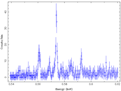
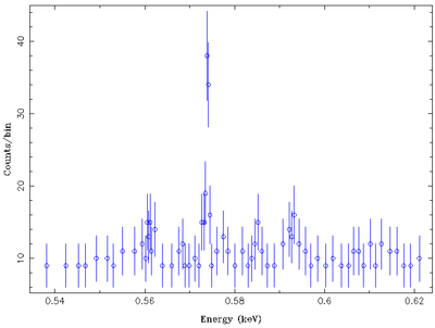
As can be clearly seen in the following two plots, which show the non-binned and the binned spectrum, while the signal to noise ratio of the data goes up, the number of bins and thus the resolution of the data goes down. This means that narrow lines can be made vanish with binning...
Exercise 1
- assuming Poisson statistics, what is the signal-to-noise ratio needed to ensure that at least 20 counts are in a spectral bin. In your estimate, assume that background is negligible.
- rebin the data set from the previous exercises to this signal-to-noise ratio and refit. Discuss how (and why) [math]\displaystyle{ \chi^2 }[/math] changes.
- (optional) An alternative to fitting data with low signal to noise is to take into account the Poisson distribution and not rebin. Instead of chi-squared-fitting, in this case one has to use the so-called
cash-statistics (named after Webster Cash who first introduced this statistics into X-ray astronomy). You can switch isis from chi-squared to Cash-statistics using theset_fit_statistic-function. Read its help and redo your fit on the unbinned spectrum using the Cash statistics. Alternatively, for moderate count rates, you can also continue using the chi-squared statistics but using the recommendations of Gehrels for the calculation of the uncertainty. Try this as well, if you are brave!
Data from multiple instruments
In previous parts of this tutorial we have already seen that when isis has loaded several spectra, these will usually be fit simultaneously. So far, however, we always applied the same spectral model to all loaded spectra when fitting the data. In many cases this is not appropriate. For example:
- Data might be from the same source, but taken during different source states. In this case, e.g., the foreground absorption might be the same, but individual spectral parameters might have to be fitted independently.
- Data might be from a simultaneous observation with different instruments. While in this case the spectral model used in fitting should be the same for all instruments, there could be slight differences in the flux calibration of these instruments. This is very typical, since flux calibration is very difficult.
This means that we need a way to distinguish between different instruments in spectral fitting. Case 2 above is by far the most common case. Here, the flux calibration can usually be taken into account by introducing a multiplicative constant in front of the spectral model that takes into account the different flux normalizations.
Exercise 2
- In the following we look at a data set of the accreting neutron star Vela X-1 that was taken in February 1996 with the Rossi X-ray Timing Explorer. The data are available at [[1]]. In the following we work with the dataset in subdirectory
gruppe05. Do the same with the data set assigned to your group.
For your information: the observation covered one full orbit of the neutron star and the absorption caused by the stellar wind of the donor star was strongly variable over the outburst. Depending on your data set you will therefore get very different answers than the ones listed here.
We first load isisscripts and the data. The internal numbers of the observations are stored in the isis variables pca, hxta, and hxtb.
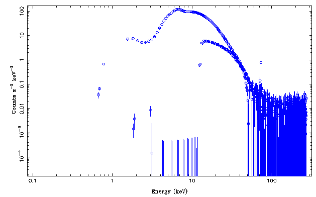
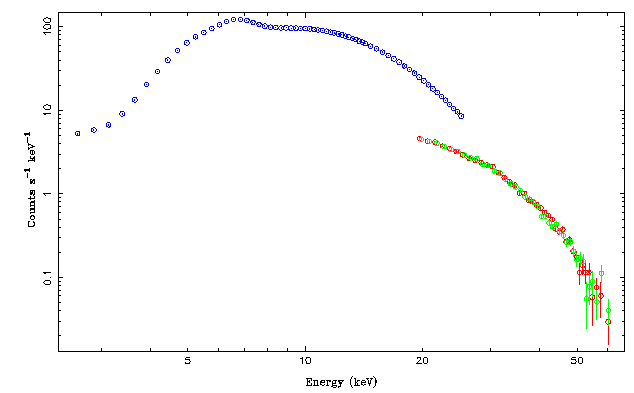
First plot the spectrum to take a look at what is available:
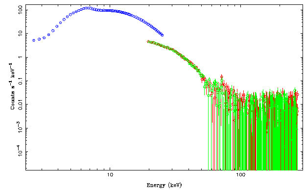
From experience we know that the PCA-data are good in 2.5-25keV, while HEXTE data are only good above 20keV. So let's ignore the data and see what the spectrum looks like:
Note that the different count rates are mainly due to the different effective areas of the instruments.
The HEXTE data are consistent with background above 100keV or so and definitively also in need of rebinning below that. We rebin both HEXTE spectra to a signal to noise of three, then plot the data and then decide to work with the 20-60keV band only
isis> group([hxta,hxtb];min_sn=3);
:
: plot etc.
:
isis> xnotice_en([hxta,hxtb],20.,60.);
This results in the following nice spectrum:
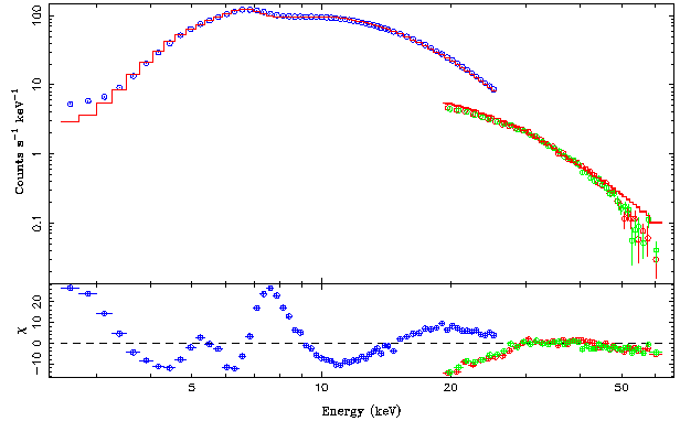
To get a better feel for what the spectral continuum looks like, let's fit a simple model. From experience we know that an absorbed powerlaw with an exponential cutoff and an iron line at 6.4keV (with some experience you can see this line in the raw data!) is generally a good empirical model for such sources. It is advisable, to first fit the model without the iron line and then add the iron line to this initial continuum. The best fit looks as follows:
isis> list_par;
phabs(1)*(egauss(1)+cutoffpl(1))
 idx  param             tie-to  freeze         value         min         max
  1  phabs(1).nH            0     0         29.52458           0      100000  10^22
  2  egauss(1).area         0     0      0.006779961           0           0  photons/s/cm^2
  3  egauss(1).center       0     1              6.4           0           0  keV
  4  egauss(1).sigma        0     0            1e-06       1e-06           1  keV
  5  cutoffpl(1).norm       0     0       0.07710349           0       1e+10
  6  cutoffpl(1).PhoIndex   0     0        0.1244691          -2           9
  7  cutoffpl(1).HighECut   0     0         10.40836           1         500  keV
isis> renorm_counts; plot_data({pca,hxta,hxtb};dcol={4,2,3},res=1);
 Parameters[Variable] = 7[1]
            Data bins = 145
           Chi-square = 8282.497
   Reduced chi-square = 57.51734
Note that the residuals are very wavy and that there is a clear offset between the PCA and HEXTE data, even though the predicted model count rate for HEXTE is much less than that for the PCA. This effect is caused by the different assumed flux normalizations of the three instruments.
In order to solve this problem we multiply each instrument with an individual normalization constant and fit these normalization constants independently of each other. In order to do so, one must know that isis evaluates the model individually for each of the loaded data sets. During the evaluation, it sets the internal isis variable Isis_Active_Dataset to the index of the data set that it is working on. This can be used to implement very complicated, instrument dependent, behavior. We now setup the model such that for each instrument we have an independent multiplicative constant:
isis> fit_fun("constant(Isis_Active_Dataset)*phabs(1)*(egauss(1)+cutoffpl(1))");
isis> list_par;
constant(Isis_Active_Dataset)*phabs(1)*(egauss(1)+cutoffpl(1))
 idx  param             tie-to  freeze         value         min         max
  1  constant(1).factor     0     0                1           0       1e+10
  2  phabs(1).nH            0     0         29.52458           0      100000  10^22
  3  egauss(1).area         0     0      0.006779962           0           0  photons/s/cm^2
  4  egauss(1).center       0     1              6.4           0           0  keV
  5  egauss(1).sigma        0     0            1e-06       1e-06           1  keV
  6  cutoffpl(1).norm       0     0        0.0771035           0       1e+10
  7  cutoffpl(1).PhoIndex   0     0        0.1244691          -2           9
  8  cutoffpl(1).HighECut   0     0         10.40836           1         500  keV
  9  constant(2).factor     0     0                1           0       1e+10
 10  constant(3).factor     0     0                1           0       1e+10
Note that we now have three multiplicative factors: constant(1), constant(2), and constant(3). Since pca has the value of 1, constant(1).factor is the multiplicative factor for the pca, and the other two constants are for HEXTE A and B.
Exercise 3
Check this claim by setting constant(1).factor to a number different from 1 and show with a few plots that the model component for PCA moves up and down while the components for HEXTE A and HEXTE B stay unchanged.
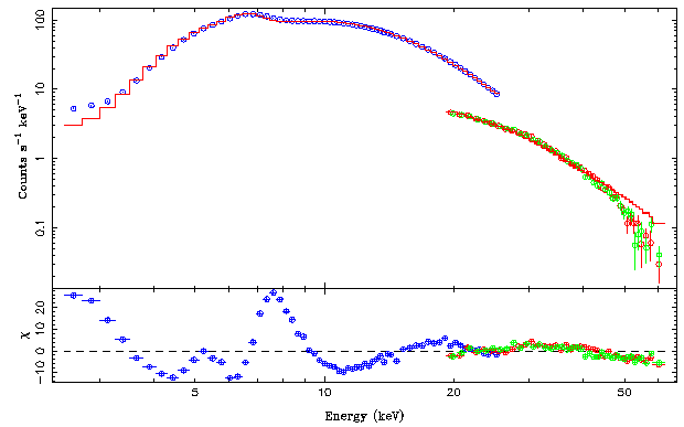
By tradition, RXTE flux normalizations are done with respect to the PCA. We therefore freeze constant(1).factor to 1 and let the other constants vary. The final fit is significantly improved with respect to our initial fit:
isis> fit_counts;
 Parameters[Variable] = 10[8]
            Data bins = 145
           Chi-square = 6471.131
   Reduced chi-square = 47.23453
0
isis> list_par;
constant(Isis_Active_Dataset)*phabs(1)*(egauss(1)+cutoffpl(1))
 idx  param             tie-to  freeze         value         min         max
  1  constant(1).factor     0     1                1           0       1e+10
  2  phabs(1).nH            0     0         30.74619           0      100000  10^22
  3  egauss(1).area         0     0      0.006348366           0           0  photons/s/cm^2
  4  egauss(1).center       0     1              6.4           0           0  keV
  5  egauss(1).sigma        0     0            1e-06       1e-06           1  keV
  6  cutoffpl(1).norm       0     0       0.09623164           0       1e+10
  7  cutoffpl(1).PhoIndex   0     0        0.2630442          -2           9
  8  cutoffpl(1).HighECut   0     0          11.7052           1         500  keV
  9  constant(2).factor     0     0          0.85297           0       1e+10
 10  constant(3).factor     0     0        0.8583705           0       1e+10
Values of around 0.85 are typical for the cross normalization of the HEXTE and the PCA. Note that in the best fit the residuals in the PCA/HEXTE region overlap rather nicely!
To make further progress with this data set, we would now need to add further features to the spectrum and life gets complicated. What works for Vela X-1 is a so-called partial covering spectrum of the form
[math]\displaystyle{ F_\mathrm{ph}(E) = \mathrm{abs}(N_{\mathrm{H},1}) (1-f+f \mathrm{abs}(N_{\mathrm{H},2})(A E^{-\Gamma}\exp(-E/E_{cut}) + g_{1} + g_{2} + b )$
\lt /latex\gt
In this model, the spectral continuum consists of two iron lines (g), the power law continuum, and a black body component (b). A fraction f of this continuum is absorbed by a large column \lt math\gt N_{\mathrm{H},1} }[/math], while all of the continuum is absorbed in addition by the foreground absorption, [math]\displaystyle{ N_{\mathrm{H},2} }[/math]. The isis implementation of this model, which takes also into account the normalization constants is as follows. Note the use of ranges (read the help for set_par) that limit the range of constant(10).factor, which is f in the above equation, to [math]\displaystyle{ 0\le f \le 1 }[/math]!
isis> list_par;
constant(Isis_Active_Dataset)*phabs(1)*(1-constant(10)+constant(10)*phabs(2))*(egauss(1)+egauss(2)+bbody(1)+cutoffpl(1))
 idx  param             tie-to  freeze         value         min         max
  1  constant(1).factor     0     1                1           0       1e+10
  2  phabs(1).nH            0     0                0           0      100000  10^22
  3  constant(10).factor    0     0        0.9770158           0           1
  4  phabs(2).nH            0     0         38.19049           0      100000  10^22
  5  egauss(1).area         0     0      0.001464248           0           0  otons/s/cm^2
  6  egauss(1).center       0     1              6.4           0           0  keV
  7  egauss(1).sigma        0     0            1e-06       1e-06           1  keV
  8  egauss(2).area         0     0      0.003165643           0           0  photons/s/cm^2
  9  egauss(2).center       0     0              7.1           0           0  keV
 10  egauss(2).sigma        0     0            0.002       1e-06           1  keV
 11  bbody(1).norm          0     0       0.01791839           0       1e+10
 12  bbody(1).kT            0     0         1.678295        0.01         100  keV
 13  cutoffpl(1).norm       0     0       0.02339737           0       1e+10
 14  cutoffpl(1).PhoIndex   0     0       -0.4117899          -2           9
 15  cutoffpl(1).HighECut   0     0         8.728334           1         500  keV
 16  constant(2).factor     0     0        0.8496358           0       1e+10
 17  constant(3).factor     0     0        0.8566091           0       1e+10
isis> renorm_counts;
 Parameters[Variable] = 17[1]
            Data bins = 145
           Chi-square = 1371.38
   Reduced chi-square = 9.523473
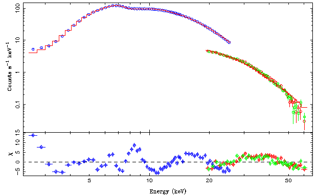
The best fit looks as follows:
Further progress with this data set could be made by using a better continuum description (an exponentially cutoff power law is a very rough approximation to the correct spectrum), but we will not do this here since the main point of this tutorial was to introduce techniques to tackle much more complicated spectral models than the ones we have encountered so far. And enough is enough...
Error Contours
In the previous part of this tutorial we already encountered the calculation of error bars using the vconf function. The approach used there is ok if there are no correlations between different fit parameters. In practice, this is rarely the case and different parameters are expected to be - sometimes strongly -correlated. The absorbed power law spectrum discussed above for Vela X-1 is a good example: At the resolution of the detector, a spectrum that is slightly steeper (higher Gamma) but slightly more absorbed (higher [math]\displaystyle{ N_\mathrm{H} }[/math]) is at some level indistinguishable from a harder, less absorbed one. Instead of talking of individual spectra it is therefore often better to look at the joint confidence contours between two (or more) parameters. The approach of calculating these contours is the same as the one used for the confidence contours for one parameter of interest, only that now we have to look at the behavior of the [math]\displaystyle{ \chi^2 }[/math]-valley for two parameters. This means that the number of fits to be performed to find the confidence range has just gone up quadratically.
However, joint confidence contours are very important and therefore isis provides an useful routine for us. To illustrate the calculation, in the following we use a simple absorbed power law to the PCA data of Vela X-1 to do the calculation. In real life, the following calculation would have to be performed on the full data set, however, we're using a simplification here to speed things up a little bit.
Since I managed to crash this writeup once, I am only giving a short introduction here in order not to stop you from doing the exercise. Please bug me to update this section later!
In isis, two-parameter confidence contours are calculated with the function conf_map_counts. The syntax of this function is as follows:
Struct_Type = conf_map_counts (Struct_Type x, Struct_Type y [, info])
where x and y are each a structure of the form
Struct_Type = struct {index, min, max, num};
listing the index of the parameter to be stepped over the range from min to max using num steps. Note that you can also use the function conf_grid(index, min, max, num) to create the above structure easily.
The help-information for conf_map_counts is very exhaustive and contains several well described examples.
Exercise
Using your above fit, write an isis-program that calculates the joint confidence contour between the absorption column and the photon index using conf_map_counts and that uses plot_conf to plot the 1sigma, 90% and 3 sigma confidence contours. Interpret the result!
