Emcee

Markov-Chain-Monte-Carlo hammer (emcee)

A Bayesian data analysis to find the probability distribution for each parameter of a model after Jonathan Goodman and Jonathan Weare. A Markov chain Monte Carlo approach has been implemented in Python by Foreman-Mackey et al., which has then been ported into ISIS by Mike A. Nowak.

Note: to access the help of any function defined in isis_emcee_hammer.sl call the function without any parameter like isis> emcee();

The common approach to find the best-fitting, or in this case the most-likely parameters of a model is to perform a χ²-minimization. Depending on the complexity of the model, finding the best-fit might take a long time or parameter degeneracies are present, which complicates the minimization process. In many cases, convergence of the χ²-minimization algorithms, such as mpfit, fails.

Another approach introduced briefly here is to ask for the probability that a certain parameter set describes the data. In particular, the probability for thousands of random parameter sets can be calculated, which results in a probability distribution not even for every single parameter, but also for the total n-dimensional parameter space.

The emcee implements such a randomized sampling of the underlying n-dimensional probability distribution. Metaphorically speaking, the idea of the Markov-Chain-Monte-Carlo approach is the following:

• use nw number of walkers for each parameter, which in the simplest case are uniformly distributed within the n-dimensional parameter space initially
• then move each walker and compare the new fit-statistic (χ²; a simple eval_counts in ISIS) with where the walker have been before
• depending on this difference, there is a certain probability that the walker goes back to its previous place
• move each walker nsim times in total

Since the choice of going back or move further is randomized as well and weighted with the fit-statistic, a worth parameter combination might get accepted. This is in contrast to the common χ²-minimization algorithms and, thus, further possible solutions within the parameter space can be found naturally. The result is the so-called parameter chain, which is a list parameters in each iteration step. The histogram of chosen parameter values is then proportional the underlying probability distribution, i.e., peaks in the distribution correspond to possible solutions. In the best case, there is only one strong peak, which corresponds to the best-fit.

Another advantage of emcee is that "[...] the MCMC basically is working off of changes in chi^2, not the absolute value. It will always give you an answer. Whether it’s a good answer in an “absolute” sense is a different question. But given your model assumptions, it will give yout the best answer." (by Mike Nowak). Or in other words, even if it is not possible to achieve a reduced χ² near 1 with a model. emcee still finds the most probable solution. Furthermore, determining parameter uncertainties in case of a bad fit-statistic is much more robust with emcee (see below).

Using emcee

This is a working minimal example with a simple power-law spectrum. First, let's fake the spectrum:

% power-law parameters
variable Gamma = 2.;
% energy grid
variable Emin = 1.; % keV
variable Emax = 10.;
variable nbins = 100;
variable lo, hi;
% fake
(lo,hi) = log_grid(Emin, Emax, nbins);
fit_fun("powerlaw");
set_par("powerlaw(1).norm", 1000);
set_par("powerlaw(1).PhoIndex", Gamma);
variable flux = eval_fun_keV(lo, hi);
variable err = sqrt(flux);
()=define_counts(
  _A(hi), _A(lo), reverse(flux + grand(nbins)*err), reverse(err)
);

Instead of perform a fit using fit_counts we use the emcee method:

emcee(
  100, % number of walkers, nw, per free parameter
  1000; % number of iterations, nsim, i.e., the number of "walker"-steps
  output = "emcee-chain.fits", % output FITS-filename for the chain
  serial % perform a calculation on a single core (see below)
);

The function does not have any return value. Also, the found best-fit is not set the chain has just been produced. To actually find the most probable parameters the resulting parameter chain has to be analyzed (see next Section).

Note: the allowed parameter ranges for the initial walker distribution is taken from the parameter ranges set in the model!

Note: the number of walkers, nw, can be much smaller than the number of iterations, nsim. However, a good value for these numbers cannot be given in general. The above example should be sufficient to have a first glance. After having analyzed the chain (see below) one might consider to change these numbers.

Warning: the output FITS-file can be extremely large (several GB), depending on the number of free parameters, walkers, and iterations! So consider writing the file to the local hard-drive (in case of a serial run) or on a network drive, e.g., userdata. In particular do not write the file in your home-directory! Analyzing the chain (see below) is comparable to a data reduction, i.e., the resulting probability distributions are much smaller in filesize.

Analyzing the chain

Note: all functions discussed here need to have the actual model defined in ISIS. Thus, after having performed the emcee run (which can take hours to days) define at least the model you have used for the emcee run (ideally there is a script which defines the data and best-fit model).

In order to read the chain-file, a function called read_chain can be used:

(nw, nfreepar, freepar, chain_statistic, chain) = read_chain("emcee-chain.fits");

Several informations are returned, such as the number of walkers, nw, the number of free parameters, nfreepar, the corresponding parameter indices, freepar, the chain_statistic, and the parameter chain itself. The chain is a 2D-matrix of doubles, chain = Double_Type[nfreepar,nw*nfreepar*nsim + x]; where the first index corresponds to the free parameter index and the second to the parameter value of a walker at a specific iteration step. The column dimension is increased by x because of [add reason here]. Thus, all values of a certain parameter, p, where the walkers "stood on", are found in chain[p,*]; This array of parameter values has to be investigated to find the most probable solution.

Paths of the walkers

First, the actual path each walker took in the parameter space should be checked. However, the column indices of the chain-matrix corresponding to the path for each walker is somehow cryptic. But one can use the chain_plot function:

close_plot; % start with a fresh plot window
_for i (0, nw-1, 1) { % loop over all walkers
                      % and plot their path
  chain_plot(
    1, % number of the free parameter (here: Gamma)
    i, % number of the walker to plot
    nw, % totalnumber of walkers
    chain; % the chain
    oplot  % overplot the window
  ); 
};

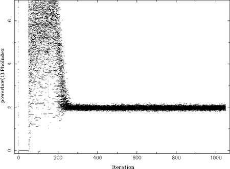
On the example plot on the right you can see how all the walkers "move" from their initial parameter value to the most probable parameter (at Gamma=2). The iteration number, i.e., the step is along the x-axis, while the y-axis shows the actual parameter value. In the beginning (at iteration 0) all walkers take uniformly distributed parameter values in the allowed range. Then all parameter values seem to be 0 for at least 50 iterations. This is, unfortunately, still a bug in emcee. Afterwards, the MCMC sets in and the paths seem chaotic as the walkers wander within the parameter space. From iteration ~250 onwards a probable value, Gamma=2, is found around which the walkers oscillate. This behavior is expected once the MCMC result has converged.

Acceptance rate

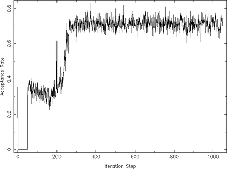
The preferred way to check the MCMC result on convergence is to investigate the so-called acceptance rate. "This is `fraction of proposed steps [of the walkers] that are accepted." ([(:biblio:ForemanMackey13)]). These steps are where the walkers did __not__ move back to its previous position (see above introduction). After [(:biblio:ForemanMackey13)] the acceptance rate should be 0.2--0.5 once the algorithm converged, although "There appears to be no agreement on the optimal acceptance rate". In order to investigate the acceptance rate of a previous emcee run, a different extension of the resulting FITS file has to be read, which can be achieved by using the frac_update-qualifier on read_chain:

frac_update = read_chain("emcee-chain.fits"; frac_update);

The returned array frac_update contains the acceptance rate at each iteration step among all walkers. Thus, by plotting this array once can easily investigate its evolution during the iteration:

 xlabel("Iteration Step");
 ylabel("Acceptance Rate");
 plot([0:length(frac_update)-1], frac_update);

In this example of a simple power-law the acceptance rate scatters around 0.7 for iteration steps higher than ~250. This resembles the behavior of the individual walkers paths we have already investigated above. This acceptance rate is, however, slightly too large, which reason is probably the very simple data and model used here. An acceptance rate close to 1 would be very similar to a random walk in the parameter space as no step is rejected. In order to avoid this issue the rejection test can be slightly tuned, which is, however, not implemented yet in the ISIS version of emcee. On the other hand very low acceptance rates (< 0.2) means "that the posterior probability is multi-modal, with the modes separated by wide, low probability valleys." ([(:biblio:ForemanMackey13)]). In this case the authors propose to split the parameter space and run an emcee for each of these regions. How to combine these runs properly is, however, not solved yet (see discussion in [(:biblio:ForemanMackey13)]).

Parameter probability distribution

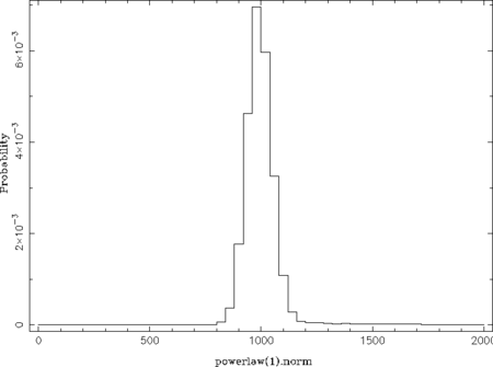
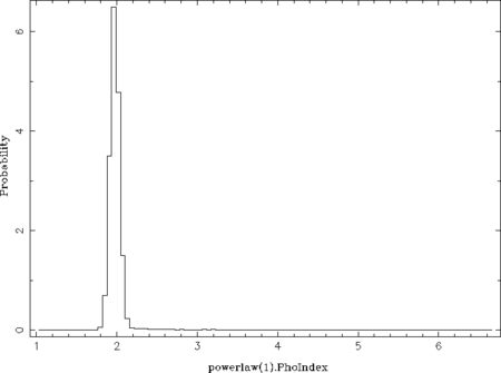
Finally, we can investigate the probability distributions of the parameters in order to find the most probable values. This requires that the emcee run converged and, in particular, the final acceptance rate is within the preferred range (which we assume to be the case for the power-law example). The probability distribution of a certain parameter is a simple histogram of the parameter values among all iteration steps, i.e., basically calling histogram(lo, hi, chain[p,*]); for the parameter p of interest. However, early iteration steps, where the acceptance rate is still to low, should be avoided (i.e., using an index array n in chain[p,n]). The function chain_hist implements these features and in case of the power-law example can be called like this:

chain_hist(
  0,          % number of the free parameter (here: power-law norm)
  chain;      % the chain
  fcut = .3,  % ignore the first fcut fraction of the data (see below)
  pmin = 0, pmax = 2000 % parameter range for the histogram (see below)
);
chain_hist(1, chain; fcut = .3, % parameter plotted here: photon index
  nbin = 100  % number of bins of the histogram
);

The qualifier fcut ignores the first fcut fraction of the data, which is set to 0.3 here as the acceptance rate is stable above iteration 300 (300./1050 ~ 0.29). The default value of 0.2 is sufficient once the total number of iterations is larger than used in this example. The qualifiers pmin and pmax control the parameter ranges used for the histogram (default: parameter ranges of the model) and nbin its number of bins (default: 50). This example results in the following two plots:

From these probability distributions one can derive the most probable parameter values by searching for the maximum (see the return_map- and return_median-qualifiers of chain_hist). This can be done in many different ways by, e.g., using a simple where_max on the histogram or by fitting the peak(s) with a Gaussian or polynomial.

Note: so far, there is no ISISscripts-function available which performs this taks because the probability distribution can be far more complicated, for instances showing several peaks. Also, the number of bins of the histogram might be adjusted in some cases.

Contours: paths in 2D

Since there is one walker for each free parameter of the model, one can not only investigate a 1D-parameter distribution, but also N-dimensional distributions (with N up to the number of free parameters). For N=2 the resulting probability distribution corresponds to the known contour maps, which can be computed by, e.g., conf_map_counts. Thus, one gets all possible contours for free using the emcee method (in the case of a large number of iteration steps). Investigating the contours might help understanding complicated 1D-parameter distributions, e.g., when multiple peaks are present.

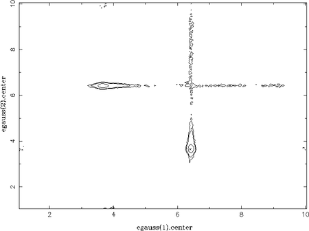
As an example, a spectrum consisting of two Gaussian lines has been faked, which are on top of a power-law continuum. Without restricting the parameter ranges for the centroid energies of the Gaussians, each line can be modelled by both components. This results in two peaks in each 1D-parameter distribution of the centroid energies (one at each line energy). Using the chain_hist2d function the contours between both centroid energies can be plotted, which nicely show these two possible solutions:

chain_hist2d(
  1,     % the x-parameter (here: egauss(1).center)
  3,     % the y-parameter (here: egauss(2).center)
  chain; % the chain
  nbinx = 300, nbiny = 300 % number of bins of the 2D-histogram
);

Like in the 1D case a histogram of the walkers (here in 2D) from the chain is calculated first. Thus, the underlying data for the contours are actually the number of walkers in each bin of the histogram. In order to derive contour levels representing certain probabilities, the function chain_hist2d calculates the minimum amount of walkers which represent these probabilities. In order to do so, the histogram is normalized to represent probabilities, i.e., the integral over the histogram is 1. Note: this means that the contour levels depend on the allowed parameter ranges! If possible (secondary) solutions are forbidden in the first place by the parameter ranges, the number of walkers in the remaining solutions are higher and, thus, the contours shrink! As it is already not trivial to derive uncertainties in case of multiple solutions (see below), the true meaning (in the sense of a significance level) of the contour lines is, however, questionable.

In order to return the contour levels calculated by chain_hist2d (for further analysis or plotting purposes) its return_cstruct-qualifier.

Interestingly, the narrow horizontal and vertical valleys in the above plot represent the path the walkers take to alternate between the two solutions. They do not move the diagonal way, which corresponds to changing the centroid energies of the two Gaussians at the same time. This is improbable because this would lead to much worse fit-statistics compared to changing only one Gaussian while keeping the other at its position. In other words, the model always fits at least one line in the data, which is not the case for the diagonal path. Furthermore, the low energy Gaussian is always moved first (there is no significant path via the lower left corner). This is because the high energy Gaussian has a higher flux and, thus, keeping one Gaussian at this energy again leads to better fit-statistics; it is less expensive to change the less significant components of the model first. This is confirmed for once the low energy line has a much higher flux: the valleys cross at the the lower left corner, i.e., at the centroid energy of the low energy line.

Chain statistics

It is also possible to investigate the actual χ² along the paths of the walkers. This data is loaded by read_chain using the chain_stats-qualifier,

(frac_update, min_statistic, med_statistic, max_statistic) = read_chain("emcee-chain.fits"; chain_stats);

which returns the minimum, median, and maximum statistics, min_statistic, med_statistic, and max_statistic, respectively, and the acceptance rate, frac_update, as described above. The three statistic arrays contain information about the χ²-distribution at each iteration step. Contrary to one might think at the first place, there are multiple evaluations of the model at each step. In detail, there is one evaluation for each walker, i.e., nw x nfreepar evaluations in total (since there are nw walkers for each free parameter, see the introduction above). Consequently, min_statistic contains the minimum value of the χ² distribution, max_statistic its maximum value, and med_statistic its median. For example, looking for the minimum within min_statistic after the MCMC converged (after iteration step 300 in the power-law example) should represent the best statistics found:

s=300; % start at this iteration step
min(min_statistic[[s:]]);

Here, this results in χ²=88.07699, which is basically identical after fitting the data, which gives χ²=88.07698. Note that you probably get slightly different values using use the above example code since faking is included. Of course, plotting the statistic array is another diagnostic tool:

n=length(max_statistic)-1;
yrange(min(min_statistic[[s:]])*.9, max(max_statistic[[s:]])*1.1);
plot([s:n], min_statistic[[300:]]);
oplot([s:n], max_statistic[[300:]]);
oplot([s:n], med_statistic[[300:]]);

Note: the χ² of the most probable solution found using emcee might be much worse (Δχ²>1) than by using a simple fit_counts. For example, this might occur for models which are describing the data qualitatively only and, thus, leading to very high χ² values in the first place. here, very narrow valleys in the parameter space might be present, where a walker simply steps. In this case, however, the emcee result still gives the most probable answer. Initializing the walkers using Gaussian distributed parameters rather than uniformly distributed ones (using the priors-qualifier on emcee, see its help) might help solving this problem.

Uncertainty estimation

In a perfect or simple case, where all probability distributions are single-peaked, the uncertainty of the most probable parameter value can be estimated by finding the parameter interval containing a certain amount of walkers, e.g., 68%. Once the distribution is multi-peaked deriving reliable uncertainties is no longer that trivial. In principle, however, finding the 68% interval for every peak while neglecting all other peaks is still okay. In this case it should be precisely described in, e.g., a paper what has been done derive the uncertainties.

In the following a code snippet for finding a certain probability interval is given in the case of a multi-peaked distribution. The idea is to first select the parameter range such that one peak is isolated:

variable p = 0; % index of the parameter of interest (here: the first free parameter)
variable lvl = .68; % confidence interval to find
variable fcut = .2; % throw away the first fcut-fraction of the chain
variable nbins = 300; % number of histogram bins

% plot the full probability distribution and let the use select
% the parameter range comfortably using the mouse
chain_hist(p, chain; fcut = fcut, nbin = nbins);
variable pmin, pmax;
(pmin,pmax,,) = cursor_box();

Then calculate the probability distribution in this parameter range and find its maximum (very simple here, you might consider fitting, e.g., a Gaussian to the peak or other functions):

% histogram to get the parameter's probability distribution
variable starti = int(ceil(fcut*length(chain[p,*]))); % start bin of the chain to use
variable lo, hi;
(lo, hi) = linear_grid(pmin, pmax, nbins);
variable hist = 1.*histogram(chain[p,[starti:]], lo, hi);
% note: no normalization here, we do that below

% find maximum (very simple here)
variable nmax = where_max(hist)[0];

In order to get rid of the continuum, which might be present in case of the paths between different solutions, we try to model it by a linear function (again, very simple):

% do a linear regression of the first and last n bins
variable n = 10;
variable ind = [[0:n-1], [nbins-n:nbins-1]];
% linear regression
variable lin = linear_regression(
  .5*(lo+hi)[ind], hist[ind]
);

% subtract the linear continuum from the probability distribution
variable newhist = hist - (lin.a + lin.b*.5*(lo+hi));
% finally, normalize!
newhist /= sum(newhist);

Finally, we determine the confidence interval by analyzing the cumulative sum:

% indices of left and right wing (undetermined index arrays; a nice SLang feature)
variable li = [:nmax], ri = [nmax+1:];
% find confidence intervals
variable conf_min = lo[li][wherefirst(cumsum(newhist[li]) > .5 - .5*lvl)];
variable conf_max = hi[ri][wherefirst(cumsum(newhist[ri]) > .5*lvl)];

The following table compares the emcee results for the power-law example above with the classical χ² approach (conf_loop([1,2], 0):

	Gamma	Norm
emcee	1.97 ± 0.06	1000 -70+90
χ²	1.97 ± 0.10	990 ± 90

As one can see, the most probable or best-fit values nicely agree within the uncertainties. The uncertainties of the emcee result seem to be slightly smaller than compared to the χ² method. This is not astonishing as the actual reduced χ² = 0.90, i.e., the fit is slightly over determined. Finding a certain Δχ² and interpreting the corresponding parameter range as an uncertainty assumes that the reduced χ² is exactly 1.

MPI emcee

=== References ===