Fit2dcurve

Fitting a curve to a 2D data set

Finding the best fit curve to a scatter plot in isis can be accomplished by combining two parameterized polynomials and using isis's minimization algorithms to "fit" the corresponding χ² value.

Here is a working example fitting a curve through the nose-like shape of the color-color diagram of Cyg X-1. First, we need to collect some data:

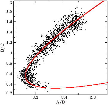
We extract the Chandra lightcurves for three energy bands: A = 0.5-1.5 keV, B = 1.5-3 keV, C = 3-10 keV. The colors we are interested in are the ratios between the count rates of two of these energy bands. In the color-color diagram we display the "soft" color AB = (0.5-1.5 keV) / (1.5-3 keV) on the x-axis, the "hard" color BC = (1.5-3 keV) / (3-10 keV) on the y-axis (see figure).

Load the data and calculate the colors:

variable a = fits_read_table("m1_0.5-1.5keV_25.5s.lc");
variable b = fits_read_table("m1_1.5-3keV_25.5s.lc");
variable c = fits_read_table("m1_3-10keV_25.5s.lc");
variable idx = where(a.count_rate >0 and b.count_rate>0 and c.count_rate>0);
struct_filter(a,idx);
struct_filter(b,idx);
struct_filter(c,idx);
variable rate = a.count_rate + b.count_rate + c.count_rate;
variable ab, ab_err, bc, bc_err, ac, ac_err;
(ab,ab_err) = ratio_error_prop(a.count_rate,a.count_rate_err,b.count_rate,b.count_rate_err);
(bc,bc_err) = ratio_error_prop(b.count_rate,b.count_rate_err,c.count_rate,c.count_rate_err);

Set up the function that returns a polynomial each for the x- and y-axis. The polynomials are parameterized via the parameter t. The order of the polynomial is determined by the number of polynomial coefficients given to the function via the array pars. In this implementation, the x and the y polynomial have to have the same order. You can obviously adjust/lift this restriction according to your needs by slightly rewriting the function.

variable t = [-1:1:0.00001];

define nosepolys(t,pars)
{
   variable np = length(pars)/2 -1;
   variable ax = pars[[0:np]];
   variable ay = pars[[np+1:2*np+1]];
   variable xt = ax[-1];
   variable yt = ay[-1];
   variable i;
   _for i(np-1,0,-1)
     {
        xt = ax[i] + t*xt;
        yt = ay[i] + t*yt;
     }
   return(xt,yt);
}

This function returns two polynomials of the form:

f(t) = coef[0] +t*(coef[1] + t*(coef[2] + t*(coef[3] ...))
     = coef[0] +t*coef[1] + t^2*coef[2] + t^3*coef[3] ...
where pars = [coef_x, coef_y] and length(coef_x) == length(coef_y)

Next, we need the fit function. Usually, isis expects a fit function fitfun(x,pars) to receive an array containing the x-values of a data set and an array (pars) listing all the coefficients of the fit function. Then, the function is evaluated on the x grid and the result compared to the corresponding y values of the data set. The fit algorithm minimizes the difference between fitfun(x,pars) and y to find the best fitting coefficients.

Since we do not have the classical y data on an x grid but rather (x,y) coordinates in a 2D map, we need to outsmart isis a little: instead of fitting the curve to the data set directly, we define the function to already return the distances of the data points to the curve. Then we minimize these distances by fitting them to a dummy x-array and a y-array consisting of a bunch of zeros. We do not care about the contents of x as long as its length equals the number of data points.

Because of the syntax restrictions for fit functions, we have no direct way to pass the real data to the fit function (using array_fit; if you are using define_counts, you can access additional information / data via set/get_dataset_metadata). We have to access them via global variables, defined above as ab, bc, and their uncertainties ab_err and bc_err. The distance of each data point is determined as the minium of the distances to each point of the parameterized curve, where the distance between two points is sqrt(Δx²+Δy²).

define nosefit(x,pars)
{
   variable xt,yt;
   (xt,yt) = nosepolys(t,pars);
   variable f = Double_Type[length(x)];
   variable i, wpar = "";
   _for i (0,length(pars)-1,1)
     {
        wpar = sprintf(wpar+" %.10f",pars[i]);
     }
   print(wpar);
   _for i (0,length(x)-1,1)
     {
        f[i] = min( ((ab[i]-xt)/ab_err[i])^2 + ((bc[i]-yt)/bc_err[i])^2 );
     }
   return f;
}

We could have done the calculation of the x- and y-polynomials within the fit function, but separating it into an extra function allows for easier plotting later.

Now we can finally fit the curve to the data set:

variable x = Double_Type[length(ab)];
variable y = Double_Type[length(ab)];
variable pars = [0.5,-2.6,4.6, 1.6,-4.6,4.1]; % start parameters

variable fres,stat;
(fres,stat) = array_fit(x,y,NULL,pars,NULL,NULL,&nosefit);
writecol(fitresdat,[stat,fres]); % save result for later

Since this implementation of this method relies on a bunch of global variables, these functions are not available through the isisscripts. Note, however, that a similar approach is available through the isisscripts: see define_xydata(), its help and references to accompanying functions therein.

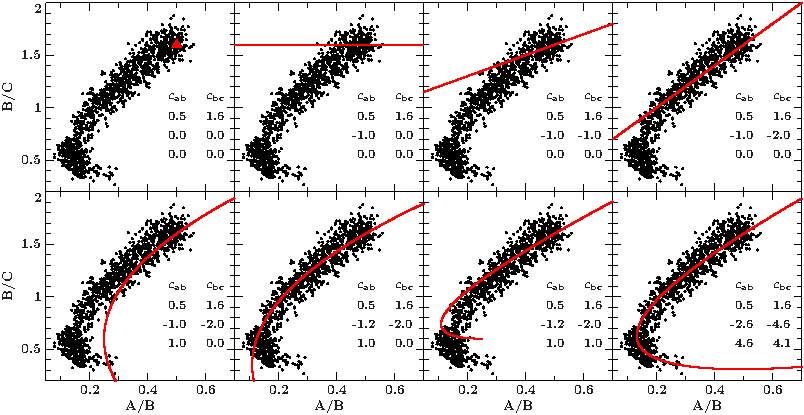
To find good starting values for the polynomial coefficients, choose a suspension point, in our example (0.5,1.6) and slowly add the subsequent parameters to get a feeling for how the curve changes (see figures). To accomplish the nose shape, polynomials of at least 2nd degree are required.

You also might have to play with the range and resolution of the parameter t.